
In this article, we will go through a comprehensive tutorial on Google Sheets Slicer. We will discuss how to apply and use a slicer in Google Sheets with some ...

In 2019, Google Sheets added one of the most in-demand tools for dashboard creation, the Slicer, in an update. While at first glance the tool may feel ...

Slicers provide a simple way to filter out data in a spreadsheet. That combined with pivot tables can provide users with a powerful data analysis tool. So, ...

While there are no direct ways, it is still possible to find the top 10 values in a Google Sheets pivot table. In this article, we will explain the ...

Percentage calculations are crucial when analyzing data. They give a clearer view of the distribution of values. We can make things even easier by taking ...
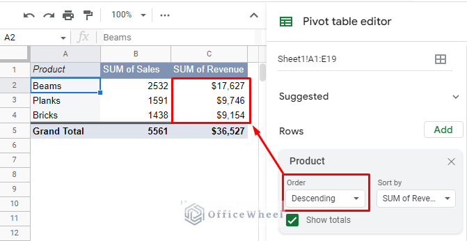
The pivot table is perhaps the most powerful data summarization tool in Google Sheets. However, we can organize it further by sorting the data by the values. ...
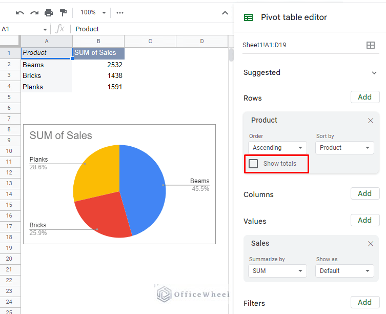
In this simple tutorial, we will show you why and how to remove the Grand Total field of a Google Sheets pivot table. Let’s get started. Why do we need to ...
With pivot tables being such a powerful data summarization tool, it is no wonder why their use is so widespread. With that popularity, many users may have ...
Pivot tables are an amazing tool when it comes to summarizing large amounts of data in Google Sheets. We can further condense our findings by grouping the data ...
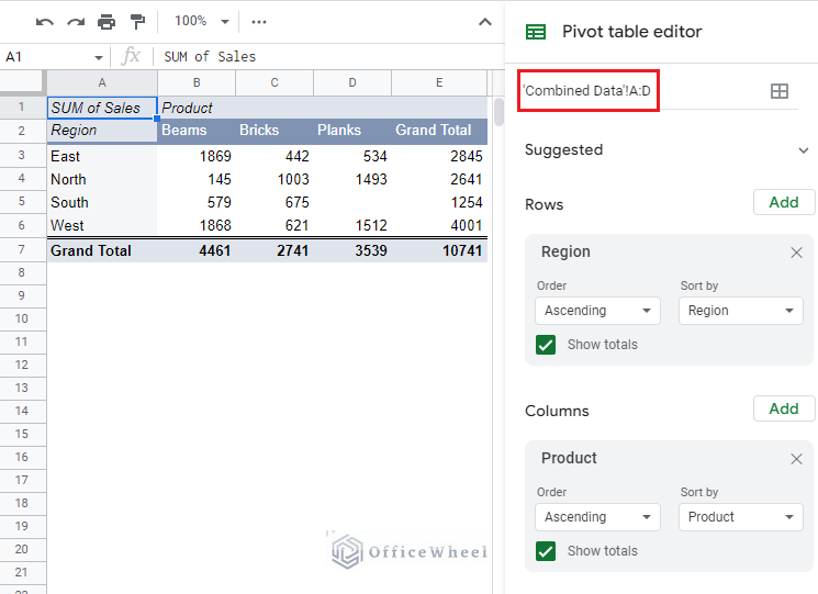
A pivot table is a powerful data summarization tool for any spreadsheet. Since it’s a spreadsheet, it is not uncommon to have data coming from multiple ...
The pivot table is a powerful tool that helps summarize large contents of data into something that is easy to derive insight from. While this tool has its ...

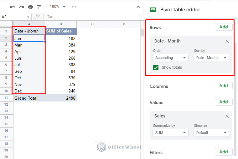
Dates can often be all over the place making it quite tough to summarize their corresponding values, even with pivot tables. However, to help with that we have ...

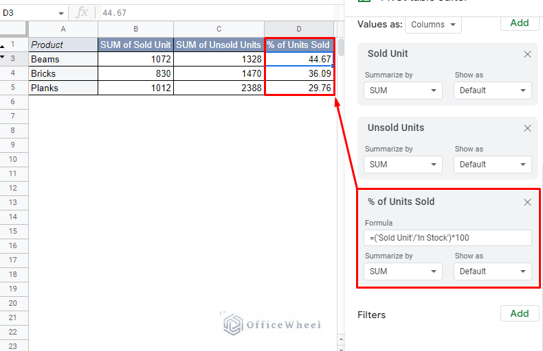
In this simple tutorial, we will look at how we can apply and utilize a Calculated Field in a Pivot Table of Google Sheets. Let’s get started. What is the ...

The pivot table is one of the most powerful tools available in a spreadsheet application. Used primarily to summarize data, pivot tables have become a staple ...
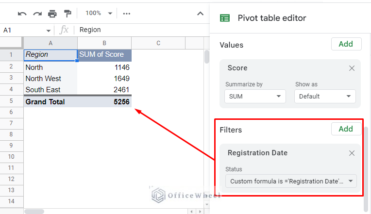
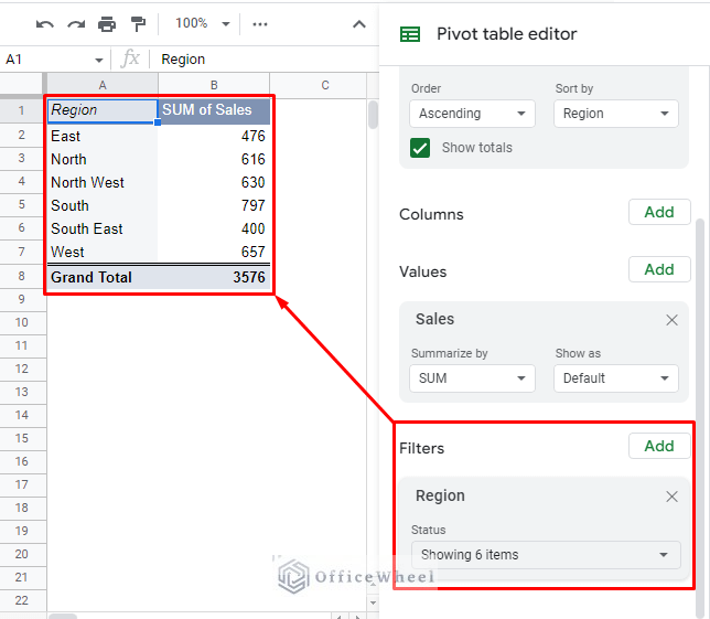
Pivot tables are perhaps one of the best data presentation tools available in any spreadsheet application. Which brings us to today’s question: Can you filter ...
- « Previous Page
- 1
- …
- 3
- 4
- 5
- 6
- 7
- …
- 14
- Next Page »
Hello,
If you want to specify which column’s changes will trigger the timestamp, all you have to do is include an IF ELSE statement inside the existing one. For example, let’s say that the SL column is Column A in the sheet:
if(sheetName == 'Stock'){
    if(range.getColumn() !== 1) return
    else{
      var new_date = new Date();
   spreadSheet.getActiveSheet().getRange(row,4).setValue(new_date).setNumberFormat("MM/dd/yyyy hh:mm:ss");
    }
}
So, if changes are made to any column other than column A or 1, no timestamps will be triggered.
For multiple triggers, we recommend different scripts for each.
I hope it helps!
Hi Max,
I am assuming that you are thinking about extracting the letters ABC from ABC-123. In this case, you can approach it in two ways without even using wildcards.
The first way is to use text functions to extract the number of characters from the string:
=LEFT(B2,LEN(B2)-4)
The LEN(B2)-4 removes the last 4 characters from the string.
For a more dynamic approach, you can look for the hyphen/dash as a delimiter to remove characters before or after it. In this case, to get ABC from ABC-123, the formula will be:
=MID(B2,1,FIND(“-“,B2)-1)
Just replace “-” with any delimiter of your choosing.
However, if you still want to extract using regular expression to get ABC from ABC-123, use this:
=REGEXREPLACE(B2,”[0-9-]”,””)
The regular expression to remove all digits and hyphens is given by [0-9-].
I hope this helps!