The pivot table is a powerful tool that helps summarize large contents of data into something that is easy to derive insight from. While this tool has its plethora of customizable options, the ability to personally customize and present data with formula is crucial in many aspects.
In this simple tutorial, we will look at a few ways that we can add and use custom formulas in a Google Sheets pivot table.
Let’s get started.
3 Ways to Add and Use Custom Formula in a Google Sheets Pivot Table
1. Include Custom Formula from the Source Dataset by Increasing the Range
It is not uncommon to have new data fields added to a dataset in Google Sheets. Especially after the original dataset is already being used for calculations or pivot tables.
For example, here we have a simple dataset:
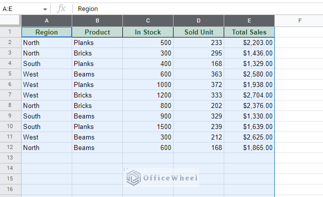
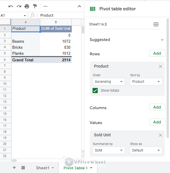
This is being used as source data for the following pivot table.
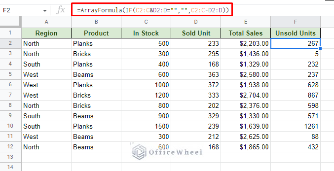
Now, let’s add a new column in the source dataset that will contain the number of Unsold Units. In column F, we enter the formula to find the number of unsold units by calculating the difference between the In Stock and Sold Unit columns:
=ArrayFormula(IF(C2:C&D2:D="","",C2:C-D2:D))The formula also accommodates blank cells.
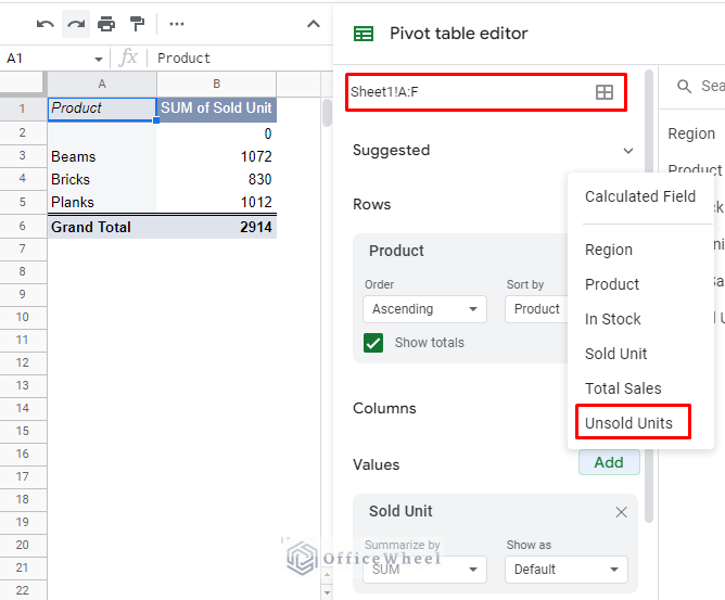
Back at the pivot table worksheet, we can’t find the column with the custom formula to add to the pivot table. This is because the range that was used to create the table did not include column F.
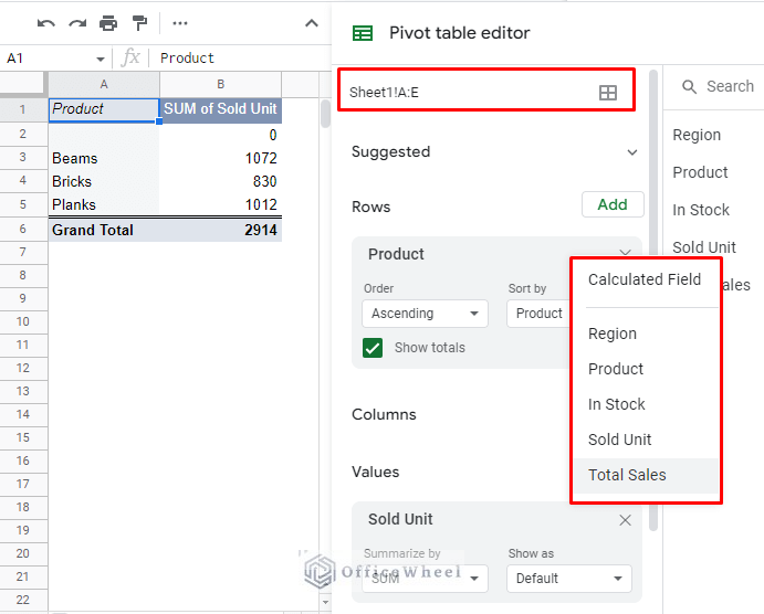
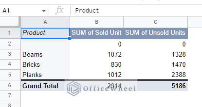
To add the column with a custom formula to the Google Sheets pivot table, we simply update the range to include column F:
The result:
2. Add Custom Formula Directly in the Pivot Table with Calculated Field
On the other hand, you may ask, can we not create custom calculations directly in the pivot table?
The answer is of course yes.
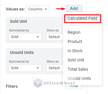
The Pivot Table Editor provides its users with an option called Calculated Field under the Values panel. This option allows users to enter custom calculations directly into the Google Sheets pivot table.
Clicking on Calculated Field will open a new panel where you can input the calculation formula. For this example, let’s say we want a column calculating the percentage of the “% of Units Sold” for each product.
=('Sold Unit'/'In Stock')*100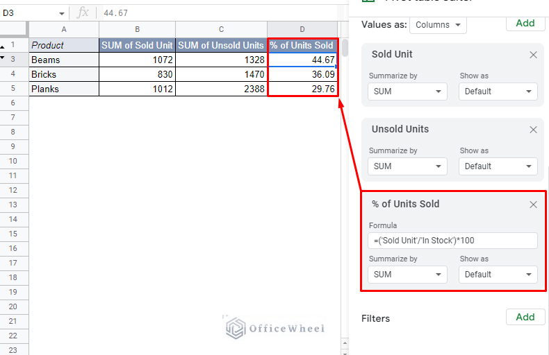
As you may have noticed, the only difference between regular formulas and pivot table formulas is how we input cell references. In a regular worksheet, we use a normal cell range reference for columns (C2:C), whereas in the pivot table we use the column header names inside single quotes (‘Sold Unit’).
Note: Some formatting was applied to the pivot table to make it look more presentable. Got rid of the empty cells and Grand Total rows and put a border around the values.
Learn More: How to Apply and Work with a Calculated Field of a Google Sheets Pivot Table
3. Filter Using Custom Formula in a Google Sheets Pivot Table
Filtering data has always been a common process for any table with data. As such, the pivot table editor has its own Filters panel.
While regular filters are available that can take care of most needs, a user may sometimes need a custom approach.
For example, let’s say we want to display the Region and Sold Unit data for Total Sales above $2000.
We have set the preliminary filter:

To set a custom condition, follow these steps:
- Click on Status.
- Filter by condition.
- Custom Formula is.
- Enter the following formula:
='Total Sales'>2000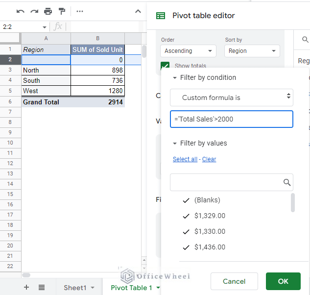
The result:
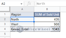
Only the North and West regions have seen sales of more than $2000.
Learn More: How to Filter with Custom Formula in a Pivot Table of Google Sheets
Final Words
As powerful a tool as pivot tables is, custom formulas can add another layer of customizability to the summarization of the data in a Google Sheets pivot table.
On that note, it is advisable to directly create calculation fields in the pivot tables instead of creating them in the source dataset. This is for the sake of efficiency.
Please feel free to leave any queries or advice you might have for us in the comments section below.