The pivot table is perhaps the most powerful data summarization tool in Google Sheets. However, we can organize it further by sorting the data by the values.
In this article, we will look at just how to do that. How to sort a Google Sheets pivot table by value.
How to Sort by Value in a Google Sheets Pivot Table
For our example, we will use the following worksheet as our source data for the pivot table:
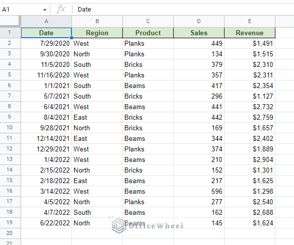
The dataset contains various data types that we will use to sort the pivot table eventually.
After creating a pivot table in a separate worksheet, we’ll have the default layout presented like this:
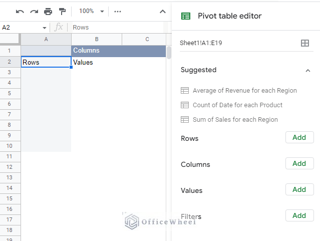
All that is left is to populate the table and show how we can sort the data in it.
Let’s get started.
1. Sort by the Value of Data in the Pivot Table
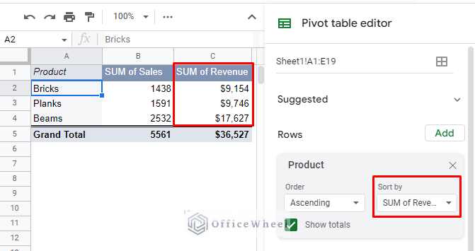
We have populated the pivot table to show the sums of Sales and Revenues for each Product:
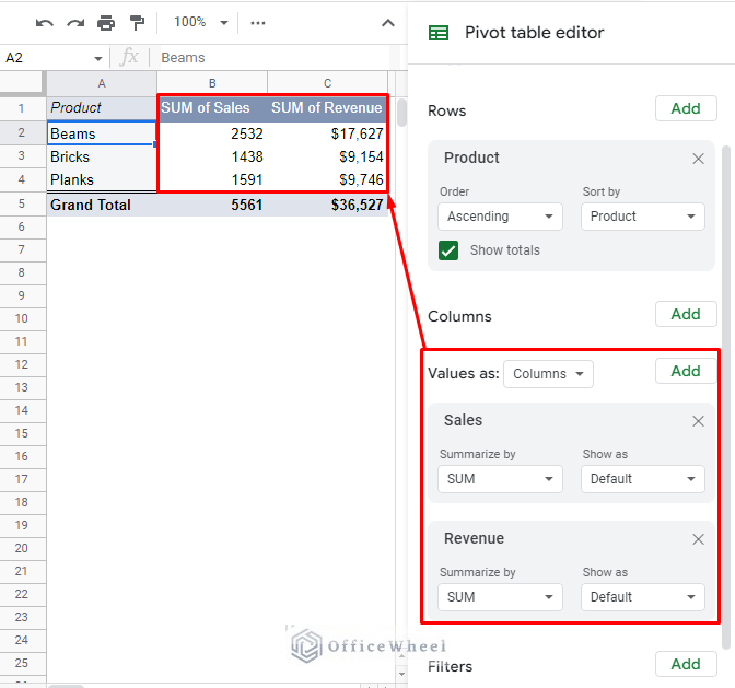
These two columns of values are important as they will be the basis of the sort. And as you can see, none of the values are sorted.
To begin, we must first decide which of these values we will use to sort the pivot table.
For this example, we have chosen the sum of Revenue.
Step 1: Go to the Rows panel and click on the ‘Sort by’ drop-down:
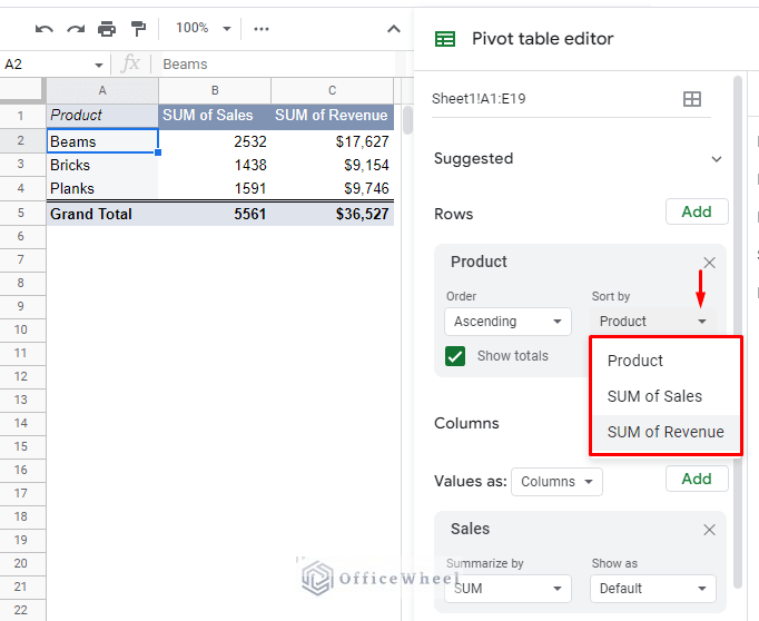
This presents all the options that are available for the user to sort the Google Sheets pivot table by.
Step 2: Select the ‘SUM by Revenue’ option to sort the pivot table by that value.
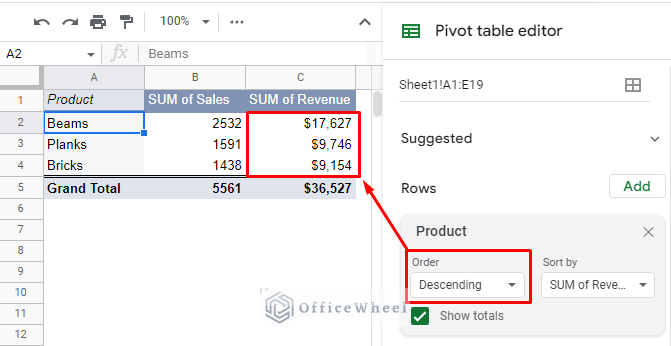
Step 3 (Optional): You can also set the order by which the table will be sorted. By default, it is set to ‘Ascending’ where the table will be sorted from the lowest to the highest value. Setting the order to ‘Descending’ will wort the pivot table from the highest value to the lowest.
2. Sort By the Value of Headers of a Pivot Table (Sort by Month)
One of the most common values used to sort any data is the Date, especially sorting data by months. The pivot table is no exception.
Here, we have created a pivot table with the primary column containing Dates that have been grouped by months. This pivot table shows the sum of sales and revenue for each month.
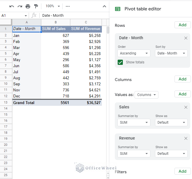
As you can see, the pivot table is already sorted in the ascending order of the month values:
A Google Sheets pivot table automatically sorts itself according to the values it is grouped by.
Which, in this case, was the month value.
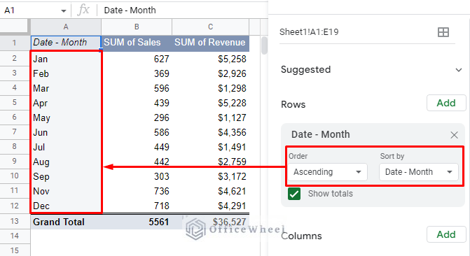
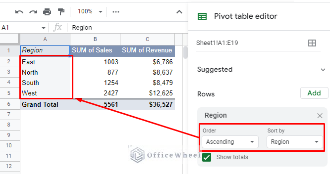
Note that Google Sheets automatically prioritizes the order of sort according to the value. In this case, month values start with January and end with December in ascending order.
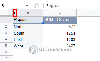
Other examples include directions and other names where the ascending order is in the alphabetical order: East > North > South > West.
3. How to Custom Sort a Pivot Table
However, if you are not satisfied with how a Google Sheets pivot table sorts your data, you can always settle for a custom sort.
For example, we know that when it comes to directions or names, the spreadsheet sorts the data in alphabetical order.
What if you wanted a custom order for this sort? Like North > South > East > West?
You can if you follow these steps:
Step 1: Create a helper column in the source dataset and input this formula in it:
=ArrayFormula(IFERROR(MATCH(B2:B,{"North","South","East","West"},0)))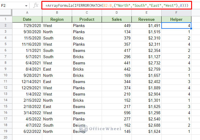
The formula looks for matching values in the Region column using the MATCH function. The function also assigns a value (1-4) to each match. This value will act as the priority of the pivot table sort.
Step 2: Update the data range of the pivot table to include the Helper column.
If you are creating a brand-new pivot table, just remember to include the Helper column.
Step 3: Add these conditions to the pivot table in order:
- Rows > Add > Helper > Deselect ‘Show totals’ checkbox
- Rows > Add > Region > Deselect ‘Show totals’ checkbox (optional)
- Values > Add > Sales
- (Optional) Filters > Add > Region > Deselect ‘Blanks’
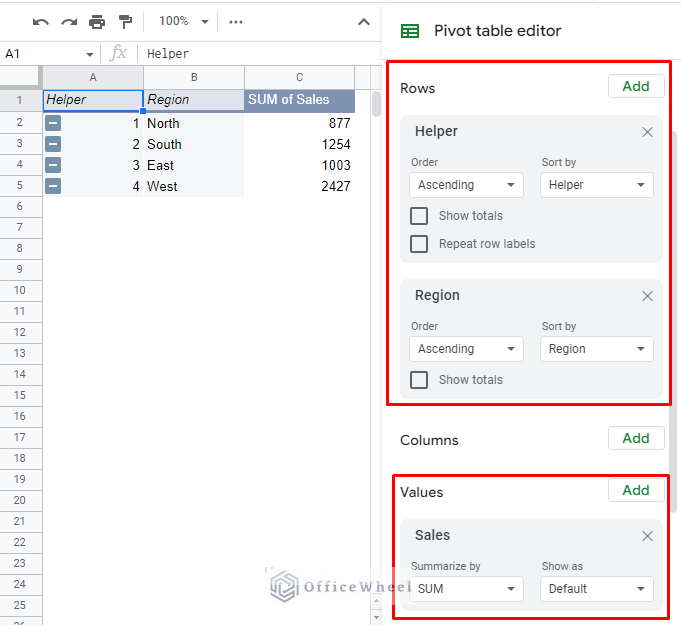
This will create a pivot table with the custom order of the Helper column, which in turn corresponds to the Region values.
Step 4: Hide the helper column from the pivot table.
And we are done!
We have successfully sorted a Google Sheets pivot table in a custom order of values.
Final Words
That concludes all the ways we can use to sort a Google Sheets pivot table by different types of values. Thanks to the pivot table editor, that task becomes that much easier. We can also take advantage of a helper column to set up a custom sort for the pivot table.
Feel free to leave any queries or advice you might have for us in the comments section below.
Related Articles for Reading
- Google Sheets Pivot Table: How to Remove Grand Total or Subtotal
- How to Apply and Work with a Calculated Field of a Google Sheets Pivot Table
- Pivot Table Formatting in Google Sheets (3 Easy Ways)
- How to Filter with Custom Formula in a Pivot Table of Google Sheets
- Using Custom Formula in a Google Sheets Pivot Table (3 Easy Ways)