Knowing how to use Wildcard characters is a great tool to possess while working in Google Sheets. Wildcards can help you maximize your search results. Being able to use Wildcards with different functions in Google Sheets is an extremely useful skill to have. In this article, we will discuss how to use Wildcard with IF condition in Google Sheets.
A Sample of Practice Spreadsheet
Download this practice spreadsheet to practice yourself.
What Is Wildcard in Google Sheets?
Wildcards are special symbols that represent a character or multiple characters in Google Sheets. They can be used to mean something when used with other functions. There are three Wildcard symbols available in Google Sheets. They are:
- Asterisk(*): Asterisk(*) represents any character or any number of characters.
- Question Mark (?): Question Mark (?) represents any single character. For example, the string ‘?ain’ could mean Rain, Pain, Gain, Main, etc.
- Tilde(~): Tilde(~) means that the preceding character should not be considered a Wildcard. This is used with other Wildcard symbols(? and *). Use this symbol(~) to tell Google Sheets to consider them(? and *) as normal characters and not as Wildcards.
3 Ways to Use Wildcard with IF Condition in Google Sheets
1. Apply Wildcard with IF Function to Get Partial Text Match
Wildcards can be used with the IF function and REGEXMATCH function for partially matching any string at the beginning, middle, or end of a text in a cell of Google Sheets.
1.1 Beginning of Text
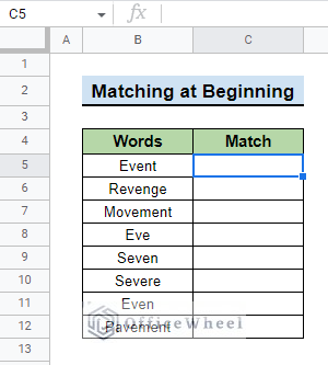
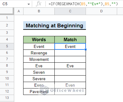
We have a table with some words in it. We want to show the words that have the letters Ev at the beginning of the words using Wildcards. Words that do not have Ev at the beginning will return an empty cell.
Steps:
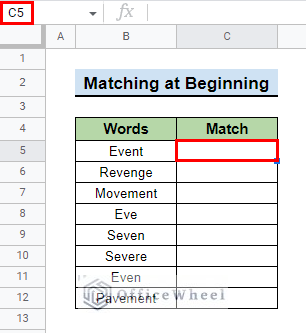
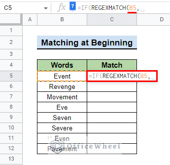
- First, go to the cell where you want to show the words containing the letters Ev at the beginning. For our example, we go to cell C5.
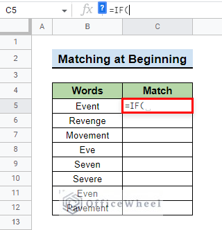
- Then, insert the IF function.
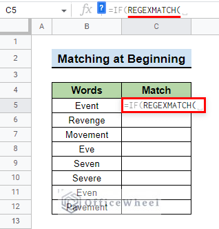
- After that, insert the REGEXMATCH function.
- Then, insert the cell number whose data you want the REGEXMATCH function to match. We type B5 for our example as this is the cell we want to match.
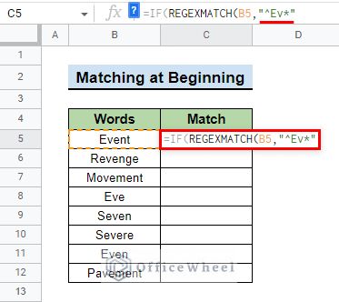
- Now, type in “^Ev*” which is the Regular Expression value for the REGEXMATCH It means to include all the characters after Ev. ^ denotes the beginning of a string. If the word does not start with Ev then it will return a blank cell.
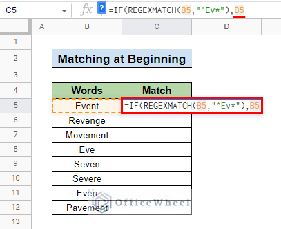
- Next, close parentheses for the REGEXMATCH function and type the value or text you want the IF function to show if the REGEXMATCH function finds a match followed by a COMMA. We want to show the text in cell B5 so we type B5 after the COMMA.
- After that, type the value or text you want the IF function to show if the REGEXMATCH function does not find a match. We type “” because we want the IF function to show a blank cell if the REGEXMATCH does not find a match.
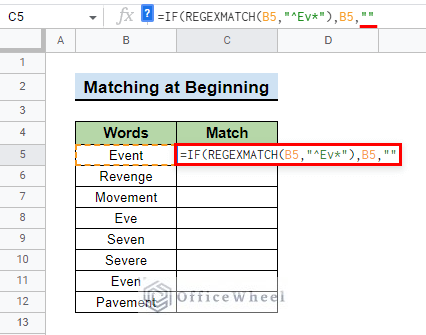
- Close parentheses and this is what the final formula looks like:
=IF(REGEXMATCH(B5,"^Ev*"),B5,"")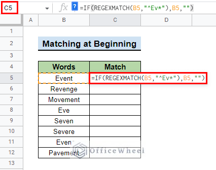
- Finally, press ENTER and drag the plus icon to have the formula copy to the below cells to have a complete table:
Read More: How to Use Wildcard in Google Sheets (3 Practical Examples)
1.2 Middle of Text
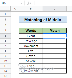
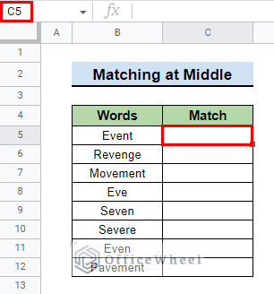
We want to use Wildcards to show the words that have the letters eve in the middle of the words. Words that do not have eve in the middle will return an empty cell.
Steps:
- First, go to the cell where you want to show the data. We go to cell C5 for our example.
- Then, type the following formula:
=IF(REGEXMATCH(B5,"^*eve*"),B5,"") 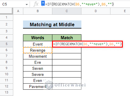
Formula Explanation:
- B5 is the cell we want to match.
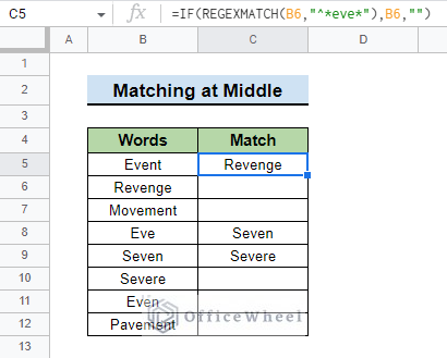
- “^*eve*” means to look for the letters eve from the start of the string till the end.
- B5 is the data we want to show if REGEXMATCH matches with the data.
- “” means if the REGEXMATCH does not find a match then the IF function will return a blank cell.
- Finally, press ENTER and drag the plus icon to have the formula copy to the below cells to have a complete table:
1.3 End of Text
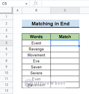
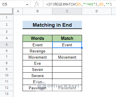
We want to show the words that have the letters nt at the end of the words using Wildcards. Words that do not have nt at the end will return an empty cell.
Steps:
- First, go to the cell where you want to show the data. For our example, we go to cell C5.
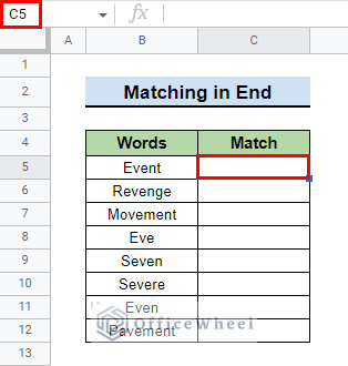
- Now, type the following formula:
=IF(REGEXMATCH(B5,"^*nt"),B5,"")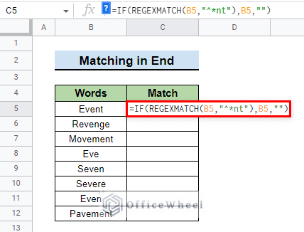
Formula Explanation:
- B5 is the data that we want the REGEXMATCH function to match.
- “^*nt” means to look for all the letters nt from the start of the string till the end.
- B5 is the text that we want the IF function to show if the REGEXMATCH function can match the data.
- “” means if the REGEXMATCH does not find a match then the IF function will return a blank cell.
- Finally, press ENTER and drag the plus icon to have the formula copy to the below cells to have a complete table:
2. Using Wildcards with SUMIF Function
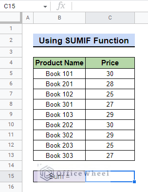
Wildcards can be used extensively with other functions such as SUMIF to have added value in calculations. Consider the dataset below. We have a list with Product names and their respective Price in a table.
We will use Wildcards to calculate different types of values from the table.
2.1 Using Asterisk (*) Wildcard
Asterisk(*) symbol can be used to represent any number of characters in the criterion part of the SUMIF function.
Steps:
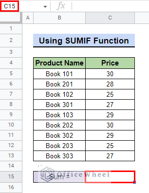
- First, go to the cell where you want the calculation to take place. We go to cell C15 for our example.
- Then, type the following formula.
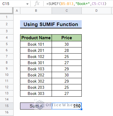
=SUMIF(B5:B13,"Book*",C5:C13)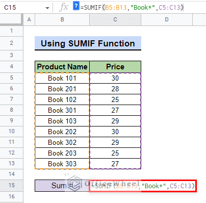
Formula Explanation:
- B5:B13 is the range of criteria that will be tested against the criteria which is “Book*” in our example.
- “Book*” is the criterion based on which the calculation will take place. The * is used to represent all the books starting with Books and ending with any characters. It takes into account Book 101, Book 102, etc.
- C5:C13 is the range that is to be summed based on the criterion specified.
- Finally, press ENTER to show the calculated sum.
- To calculate the price of Books starting with 2, type the following formula.
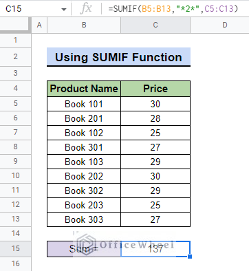
=SUMIF(B5:B13,"*2*",C5:C13)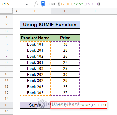
- Asterisk(*) sign before and after 2 means the SUMIF function will take into account all the characters before and after 2.
- To calculate the price of Books ending in 3 use the following formula.
=SUMIF(B5:B13,"*3",C5:C13)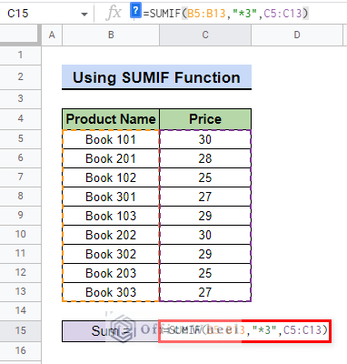
- Asterisk(*) before 3 means the SUMIF function takes into account all the characters before 3.

2.2 Utilizing Question Mark (?) Wildcard
Question Mark(?) can be used to indicate any single character in the criterion part of the SUMIF function.
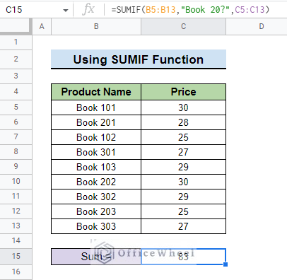
- Type the following formula to calculate the sum of the price of all the books starting with 20 and ending in any one character i.e. 1, 2, 3.
=SUMIF(B5:B13,"Book 20?",C5:C13)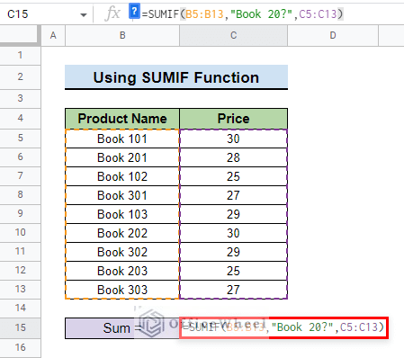
- ? represents any character that is after 20.
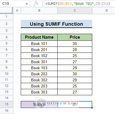
- We can even calculate the sum of the price of Books ending in 03 by using the following formula.
=SUMIF(B5:B13,"Book ?03",C5:C13)
- Press ENTER to show the result.
2.3 Applying Tilde (~) Wildcard
If we have any of the above two symbols in our dataset then we can use Tilde(~) to consider them as normal characters rather than wildcards.
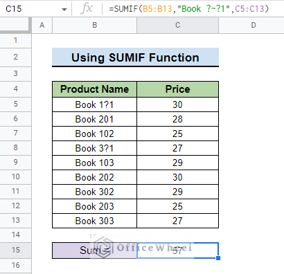
- Let’s say we have the following dataset with Question Mark(?) in place of 0.
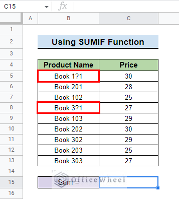
- We can calculate the sum of the price of the books with the following formula.
=SUMIF(B5:B13,"Book ?~?1",C5:C13)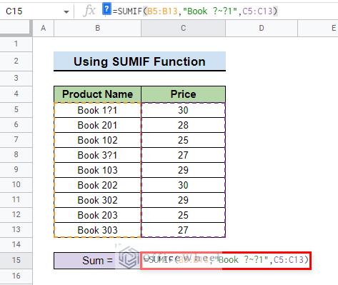
- Here, the first ? represents character 1 or 3 in this case. Tilde(~) denotes that the character adjacent to it is a normal character. Meaning, the second ? has to be considered a normal character by the SUMIF function.
3. Utilizing Wildcards with COUNTIF Function
Wildcards can be used with the COUNTIF function to partially match the data and count their occurances. This method is very useful when you want to partially match data and show the count.
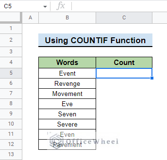
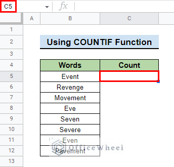
Suppose we have a dataset with a list of words and we want to know all the words that contain the letters eve in them. To find this out, we have to use Wildcards with the COUNTIF function.
Steps:
- First, go to the cell where you want to show the count. We go to cell C5 in our example.
- Then, type the following formula:
=COUNTIF(B5:B12,"*eve*")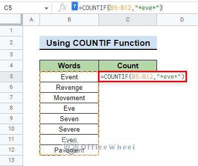
Formula Explanation:
- B5:B12 is the range where we want to test against the criterion, which is the letters eve in this case.
- “*eve*” is the criterion based on which the formula will find the words in the range and count them. The Asterisk(*) before and after eve means that the formula should consider all the characters before and after eve to find a match.
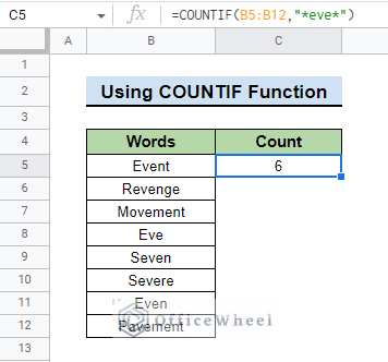
- Finally, press ENTER to have your count.
Conclusion
In this article, we showed you how to use Wildcards in Google Sheets in 3 different methods. Keep practicing the methods along with the examples that we have shown here for a better understanding of the concept. We hope this article was useful to you.
Also, check out other articles on OfficeWheel to keep on improving your Google Sheets work knowledge.