How to Use SUMIF Function with Wildcard in Google Sheets

This article covers how to use the SUMIF function with wildcard to sum cells based on criteria in Google Sheets. You may sum cells based on a variety of criteria with text, numbers, and dates. Using wildcards makes the criteria more dynamic. This also helps to keep the formulas neat and concise. Today, we’ll take a closer look at using wildcards with the SUMIF function.

Table of Contents

What Is Wildcard in Google Sheets?

Wildcards are special characters in Google Sheets that are used to represent other characters. They are very useful while entering criteria for conditional functions (SUMIF, COUNTIF, etc) or searching for approximately matching strings in Google Sheets.

Usually while using Google Sheets to make calculations, we need to determine the exact string that should go into the formula. Moreover, we may need to search for values that may include any particular string. Fortunately, in both cases, Google Sheets wildcards can be of great benefit. To assist you to find the most relevant search results possible, wildcards are special symbols that can represent one or more string characters. You can use the following 3 wildcards in Google Sheets.

The Asterisks(*): This character can take on any number of forms.
Question Mark(?): A single character is symbolized by this wildcard.
Tilde(~): This wildcard is used to instruct Google Sheets that the following character should not be treated as a wildcard but rather as a regular character symbol. It is typically used before one of the above wildcard characters. (* or ?).

6 Examples of Using SUMIF Function with Wildcard in Google Sheets

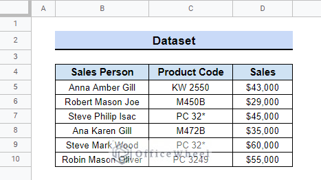
Now, you can have a look at our dataset which contains three columns including Sales Person, Product Code, and Sales. In this article, we will show you how to use the SUMIF function with wildcard to get the sum of sales based on different criteria.

Follow the examples below to learn how to do that.

1. For Partial Match

1.1 Beginning of Name

Suppose you need to find the total sales made by the salespersons whose names start with certain characters. You can use the Asterisks(*) wildcard after the characters in the criteria of the SUMIF function to do that. Here is the example below:

Consider you need to get the sum of sales made by Sales Persons whose names start with Steve. Here, two of the salesperson’s names start with “Steve”.

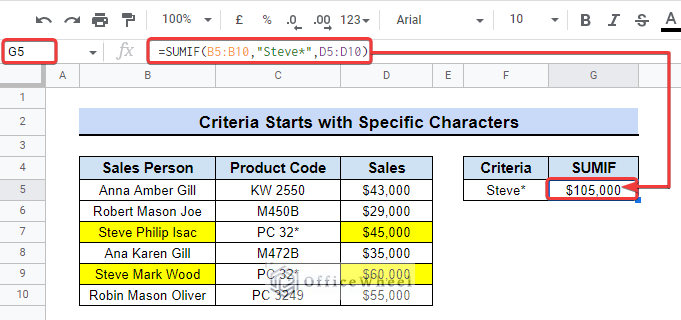
Then you can just apply the following formula in cell G5 to get the desired output as shown below.

=SUMIF(B5:B10,"Steve*",D5:D10)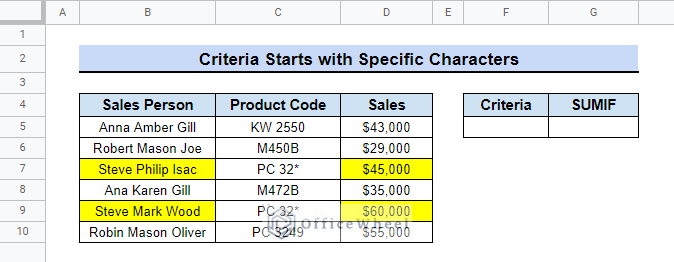

Here we use the asterisks(*) wildcard after Steve as Steve* to suggest that the name must start with Steve and the rest of the characters can be anything. Also, notice that the criterion is enclosed with double quotes as “Steve*”.

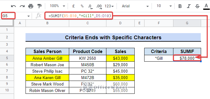
1.2 End of Name

Now assume you need to find the total Sales made by the Sales Persons whose names end with certain characters. You can use the Asterisks(*) wildcard before those characters in the criteria of the SUMIF function to do that. Here is the example below:

Consider you need to get the sum of sales made by salespersons whose names end with Gill. Here, two of the salesperson’s names end with “Gill”.

Then apply the following formula in cell G5 to get the following result.

=SUMIF(B5:B10,"*Gill",D5:D10)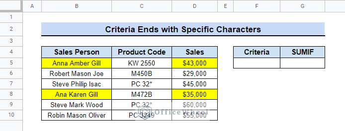

Here we use the Asterisks(*) wildcard before Gill as *Gill to suggest that the names may begin with any number of characters. But it must end with Gill.

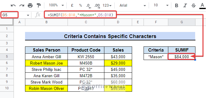
1.3 Middle of Name

You can also use the asterisks(*) wildcard to sum Sales made by salespersons with a particular middle name. You need to use the * wildcard before and after the middle name in the criteria for that.

Suppose you want to get the total sales by a salesperson whose middle name is Mason. The dataset contains two such cells as highlighted below.

Then enter the following formula in cell G5 to get the result below.

=SUMIF(B5:B10,"*Mason*",D5:D10)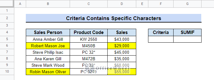

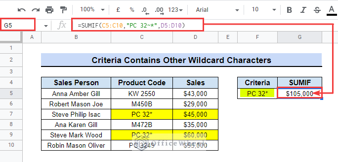
2. Criteria Contain Wildcard Characters

Now suppose you need to find the total sales of particular products whose Product Codes contain certain wildcard characters. Then you need to use the Tilde(~) wildcard before that wildcard character in the criteria of the formula. Here is the example below:

First, have a look at our dataset. Assume you want to sum the sales for the product code PC 32*. If you directly use this as the criteria in the formula, it will also sum the sales for PC 3249.

You need to use the Tilde (~) wildcard before the * in the criteria. This is to verify that the * itself is a normal character rather than a wildcard. Apply the formula in cell G5 to see the desired result.

=SUMIF(C5:C10,"PC 32~*",D5:D10)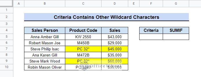

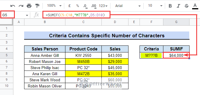
3. Have Specific Number of Characters

In this example, we will highlight how to sum the Sales if the Product Codes contains a specific number of character in specific positions. You need to use the Question Mark(?) wildcard in the criteria to do that.

Consider you need to get the total Sales for Product codes starting and ending with M and B, and containing any three-digit numbers in between them. Here, M450B and M472B contain match those criteria.

You need to use 3 question marks (?) as the wildcard in the criteria of the formula. Apply the following formula in cell G5 to get the following output.

=SUMIF(C5:C10,"M???B",D5:D10)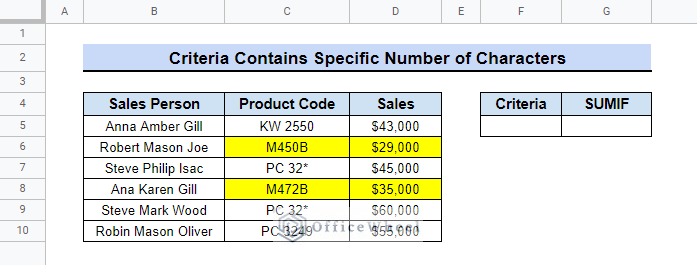

4. Criteria with Wildcard and Cell Reference

Now, we will highlight using the SUMIF function with wildcard and cell reference in Google Sheets. Suppose, you want to know the sum of the sales of a salesperson with similar middle names. Have a look at our step-by-step procedure below.

Consider you need to get the total Sales for Sales_Person having a similar middle name “Mason”, so we highlighted the cells containing this name.

Then, we use Mason as criteria and get the formula using a wildcard with cell reference in the SUMIF formula. Here, we use cell F5 as a reference.

=SUMIF(B5:B10,"*"&F5&"*",D5:D10)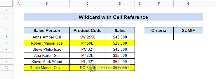

As we use cell reference, after that, if we want to get other values, we can just change the criteria in cell F5 and the sum of the values will update automatically. Here, the formula is slightly changed as these names contain the specific character at the end, so we will refer first part using asterisks(*) and for the remaining part we will use a cell reference.

=SUMIF(B5:B10,"*"&F5,D5:D10)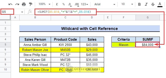

Things to Remember

Put the criterion in quotation marks if it contains text, a wildcard character, or a logical operator that is then followed by a number, text, or date.
Use quotation marks to introduce a text string and an ampersand (&) to concatenate and end it if the criterion calls for both a logical operator and a cell reference or another function.

Conclusion

In this article, we have discussed how to use the SUMIF function with wildcard in Google Sheets. Here, we have mentioned 6 examples of how you can use wildcards along with SUMIF to get the sum result of a specific range. We hope, it was helpful to you. Please, don’t forget to visit our OfficeWheel website to know more details about Google Sheets to make your work easier. Leave a comment if you have more examples to do this and if you faced any problems understanding any of the examples we mentioned.