Reference Another Sheet in Google Sheets (4 Easy Ways)

Today, we look at how to reference another sheet in Google Sheets. While it does sound easy (and it is), it’s common to see users of all levels of spreadsheet expertise mess up.

This article stands as a trusty guide for those situations. Let’s get started.

Table of Contents

Reference Another Sheet in the Same Spreadsheet in Google Sheets

1. Basic Cell Reference to Another Sheet

To show our processes, we have created this workbook containing worksheets of three separate workplaces: Office 1, Office 2, and Office 3. And a fourth worksheet called Master List which we will be populating.

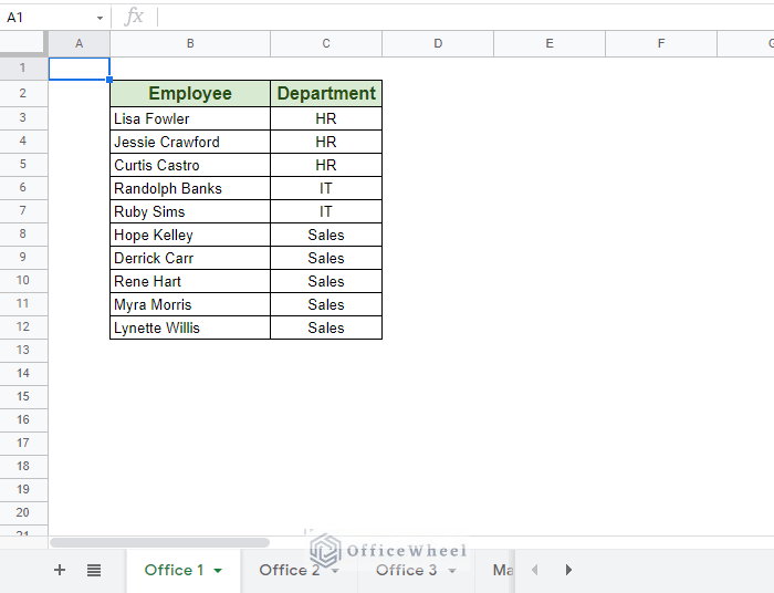
Office Worksheet

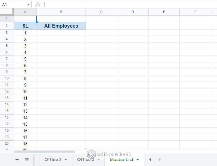
Master List Worksheet

a. Single Cell Reference from Another Sheet

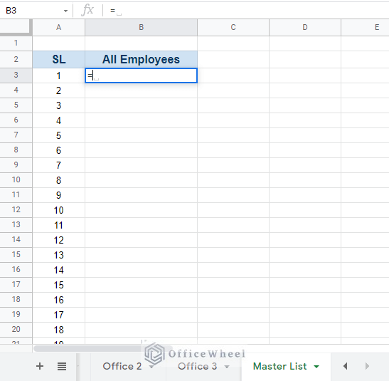
Let’s start simple. We will be extracting (referencing) the name of the first employee from Office 1 worksheet to cell B3 of the Master List worksheet.

Step 1: Input equals-to (=) in cell B3.

Step 2: Move to Office 1 worksheet and select the first name there.

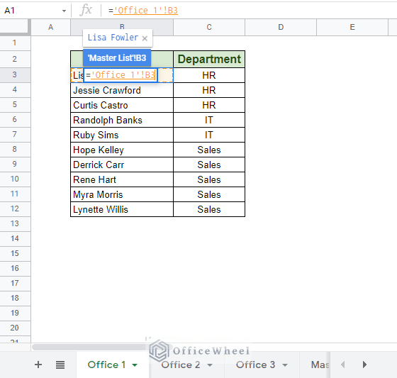
Step 3: Press ENTER.

='Office 1'!B3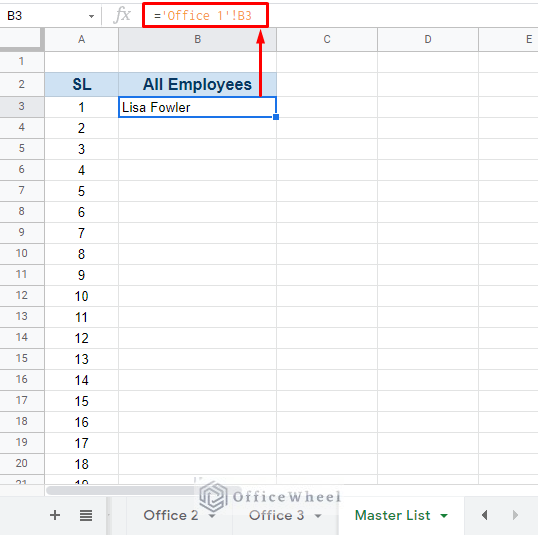

You can also type in the name of the worksheet you are referring to within single quotes (‘’) and the cell number of that worksheet separated by an exclamation (!).

Thus, our syntax for referencing another worksheet in Google Sheets is:

='worksheet-name'!cell-reference

b. Range Reference from Another Sheet in Google Sheets

Range references work the same way. Instead of typing in a single cell value, we input a range.

Continuing from Step 2 from our previous section, we click and drag down the column of names to select them.

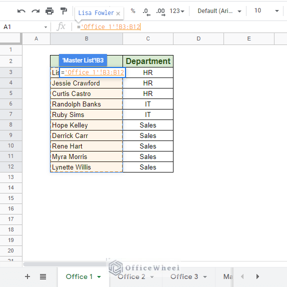
Press ENTER.

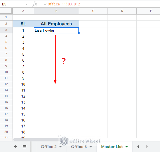
But this doesn’t show all the names, does it?

The data has been extracted but it is confined to one cell. To display all the names we have to present the data as an array, thus we have to enclose the formula within curly braces {}.

={'Office 1'!B3:B12}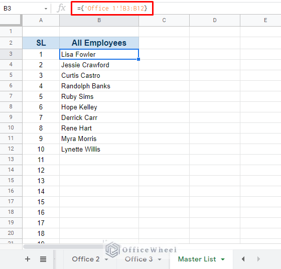

That concludes the fundamentals of referencing data from another sheet in Google Sheets. From this point onward, we will be looking at the iterations of what we have learned, up to referencing another spreadsheet entirely.

2. Import Data From Multiple Sheets into One Column

A situation may arise where you may need to extract data from ranges that belong to multiple worksheets. Similar to our All Employees column in our Master List worksheet, where we want to list the names of all employees from the three offices.

To help us with that, we will utilize the FILTER function.

To extract names from Office 1 we use the following formula:

=FILTER('Office 1'!B3:B12,LEN('Office 1'!B3:B12)>0)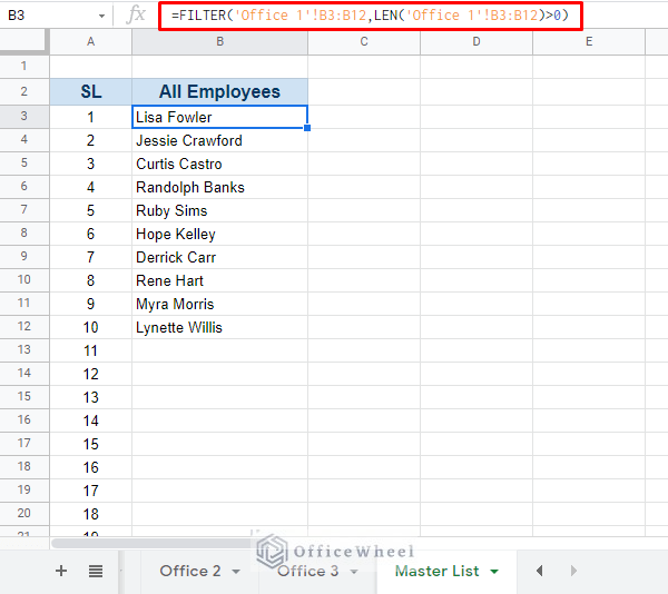

Formula Breakdown:

‘Office 1’!B3:B12: Our range of names in the Office 1 worksheet. You can update the range to ‘Office 1’!B3:B to extract the column dynamically.
LEN(‘Office 1’!B3:B12)>0: Our condition for extraction. It checks whether the value of the cell is greater than 0, returns TRUE if it is.

This formula functions similarly to ={'Office 1'!B3:B12} of the previous section, up to the point of outputting the data as an array.

Formula for Office 2:

=FILTER('Office 2'!B3:B,LEN('Office 2'!B3:B)>0)

Formula for Office 3:

=FILTER('Office 3'!B3:B,LEN('Office 3'!B3:B)>0)

All we need to do now is combine the different sections with a semicolon (;) separator and enclose it in curly braces {}:

={FILTER('Office 1'!B3:B,LEN('Office 1'!B3:B)>0);FILTER('Office 2'!B3:B,LEN('Office 2'!B3:B)>0);FILTER('Office 3'!B3:B,LEN('Office 3'!B3:B)>0)}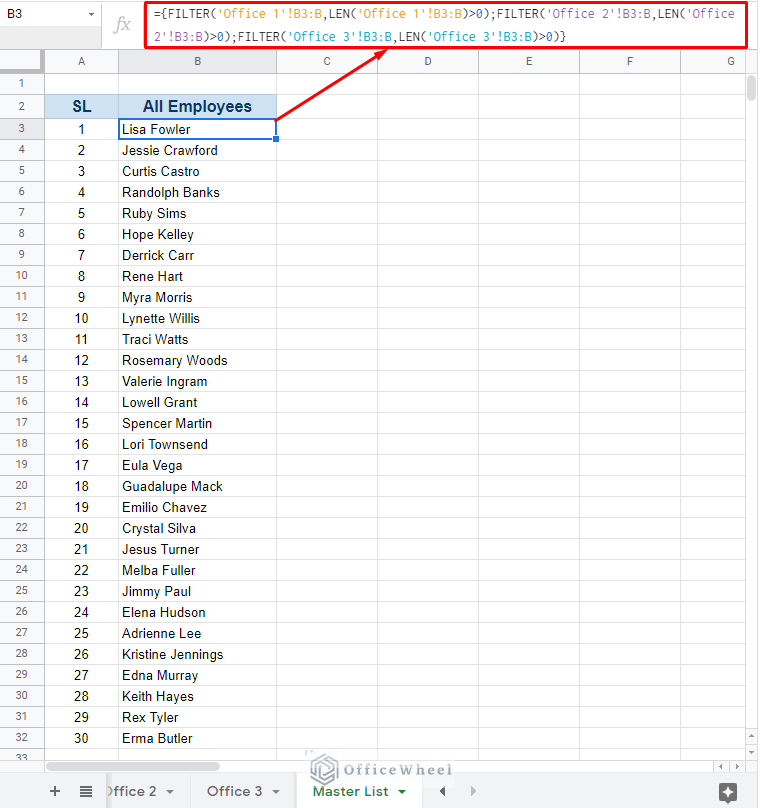

One other advantage of using this method is that it is dynamic. Not only for new data added to each of these Office worksheets but also for the worksheet names. So even if you change the name of the worksheet, it will be reflected in the formula.

dynamically adding new items to the list animated

Adding a new Employee Name

Changing the worksheet name also changes its name in the formula

Similar Readings

3. Import Data With Criteria

To present this method, we will again use the FILTER function, but we will be changing up the scenario.

This time, we will extract names according to the Departments of the Employees.

The modification to the formula is simple:

=FILTER(‘Office 1′!B3:B,’Office 1’!C3:C=”Sales”)

Source worksheet: Office 1

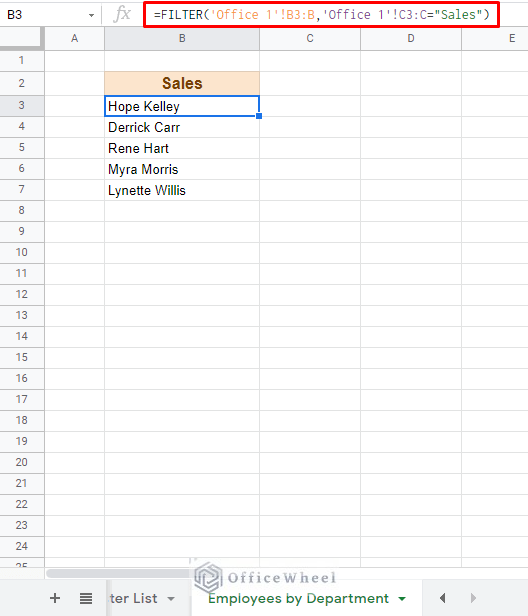
You can do it for all the departments. The Department name condition can be referred to the header cells.

=FILTER('Office 1'!$B$3:$B,'Office 1'!$C$3:$C=C$2)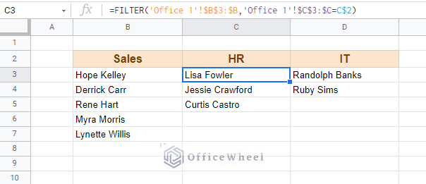

Reference Another Sheet From a Different Spreadsheet in Google Sheets

Google Sheets does not restrict us to only reference worksheets from the same spreadsheet. We can also use references from a separate spreadsheet thanks to the IMPORTRANGE function.

The IMPORTRANGE syntax:

IMPORTRANGE(spreadsheet_url, range_string)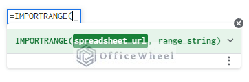

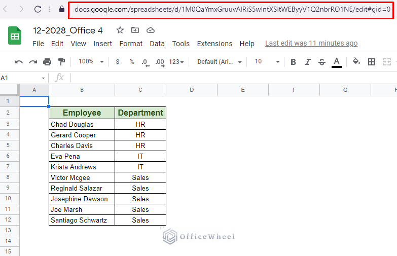
We have created a separate workbook containing the Office 4 worksheet

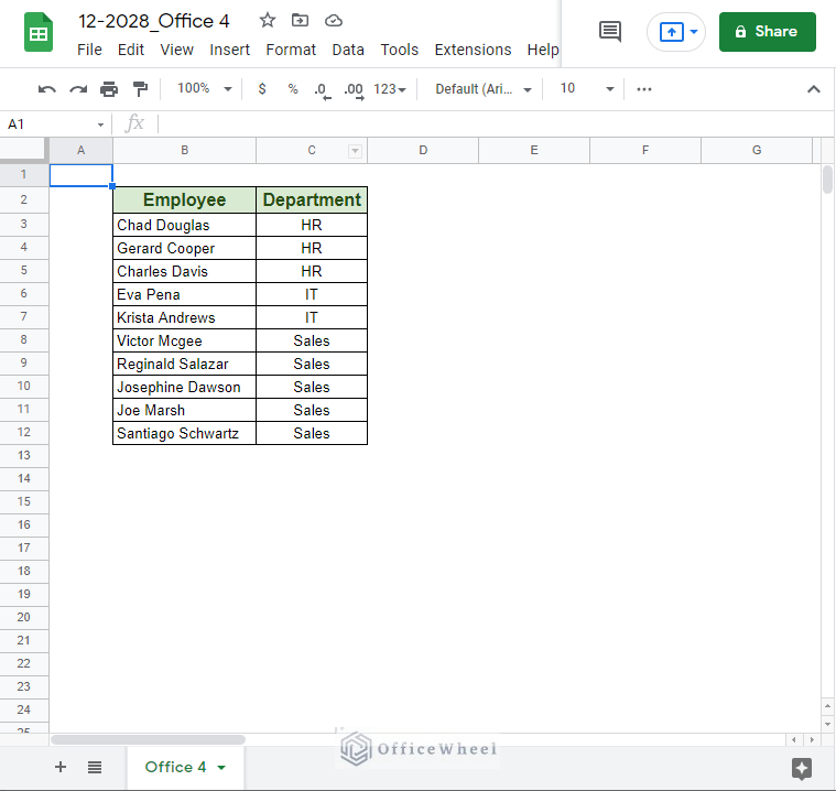
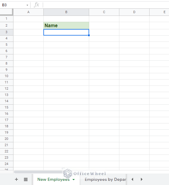
We will be extracting all the names from the Office 4 spreadsheet here in the New Employees worksheet in our main workbook.

Let’s go through the process, step-by-step.

Step 1: Open the function in cell B3, =IMPORTRANGE(

Step 2: Copy the URL of the other workbook and paste it within the function within quotation marks (“”). Press comma (,) to move to the next part

Step 3: Input the worksheet name and the range of cells in the following format:

“Office 4!B3:B12”

Step 4: Close parentheses and press ENTER.

=IMPORTRANGE("https://docs.google.com/spreadsheets/d/1M0QaYmxGruuvAlRiS5wlntXSltWEByyV1Q2nbrRO1NE/edit#gid=0","Office 4!B3:B12")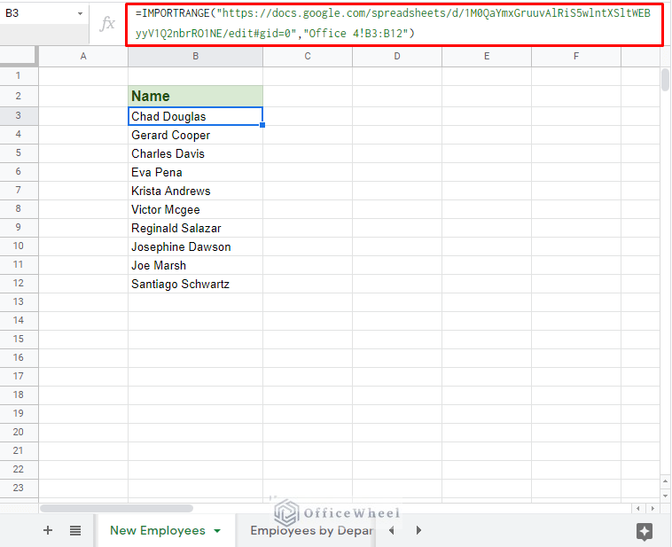

Alternatively, we can also use the Spreadsheet Key of the spreadsheet URL in the formula to give the same results.

Spreadsheet Key

New formula:

=IMPORTRANGE("1M0QaYmxGruuvAlRiS5wlntXSltWEByyV1Q2nbrRO1NE","Office 4!B3:B12")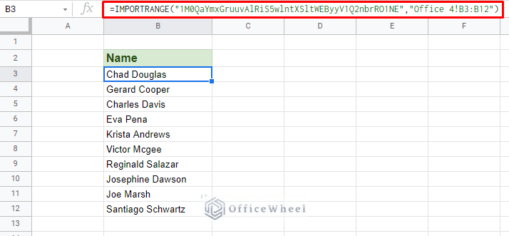

If you want to learn more, here’s an in-depth guide on How to Reference Another Workbook in Google Sheets.

Final Words

The ability to reference another sheet in Google Sheets is very easy. The only difference you may face, when compared to applications like Excel, is when we reference a different workbook or spreadsheet entirely with its IMPORTRANGE function.

We hope that the methods we have presented in this article help to solve any issues you may face or to just simply understand how referencing works in Google Sheets.

Feel free to leave any queries or advice you may have for us in the comments section.