Reference Another Workbook in Google Sheets (Step-by-Step)

Contrary to popular belief, barring certain confusing aspects of spreadsheets, how to reference another workbook in Google Sheets is fairly simple.

We are going to show you how to do so in easy progressive steps in this article. Let’s get started.

Easy Steps to Reference Another Workbook in Google Sheets

To show you the process of referring to another workbook and extracting data from them in Google Sheets, we have created a particular dataset in the Class Details spreadsheet.

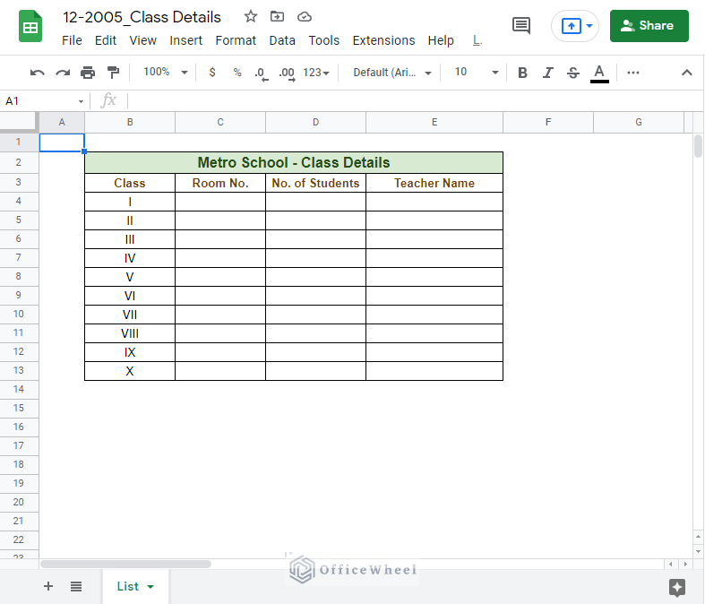
In this workbook, we have a table that will contain all the classroom information of Metro School. But our data is in two other spreadsheets.

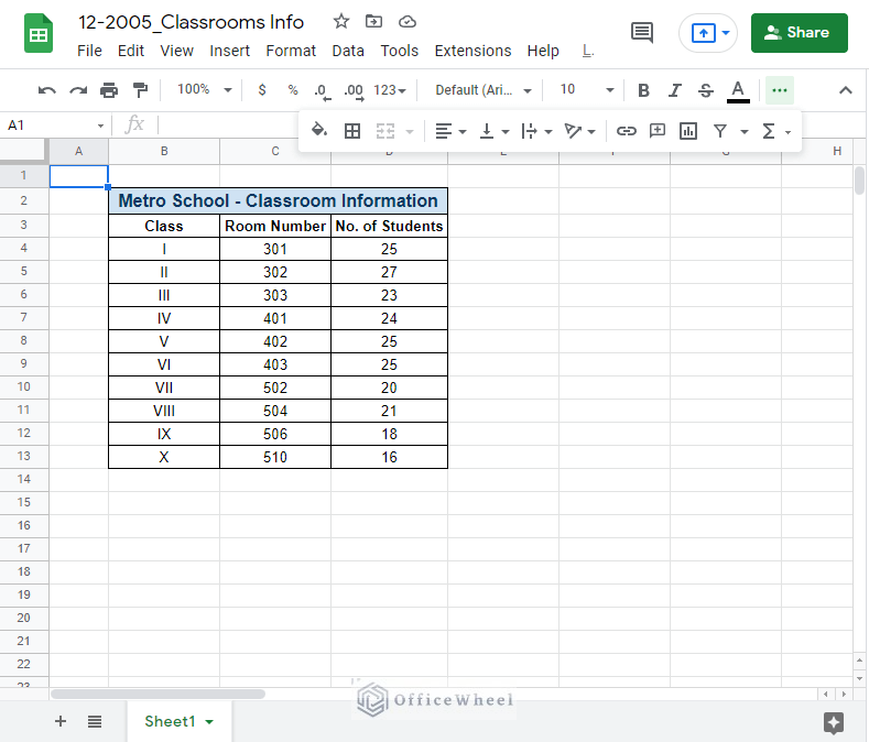
Classroom Info Spreadsheet

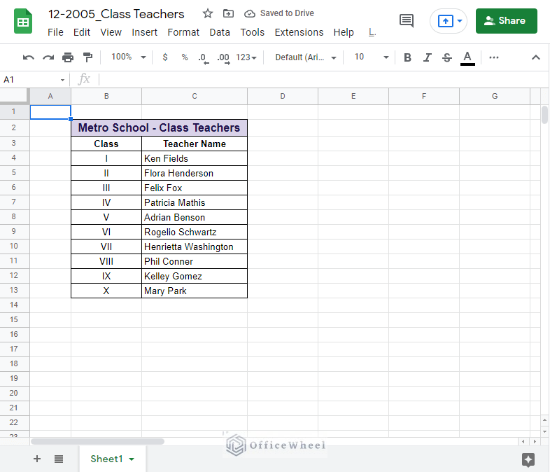
Class Teachers Spreadsheet

We are going to be extracting these data from the different workbooks and organizing them together in a single one, the Class Details spreadsheet. We can do this thanks to the IMPORTRANGE function.

The syntax of IMPORTRANGE is:

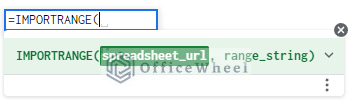
• spreadsheet_url: The URL of the other spreadsheet/workbook in Google Sheets from which you are going to extract your data.
• range_string: contains the name of the worksheet of the other workbook and the range of cells containing desired data.

Note: Both spreadsheet_url and range_string must be enclosed within quotation marks (“”).

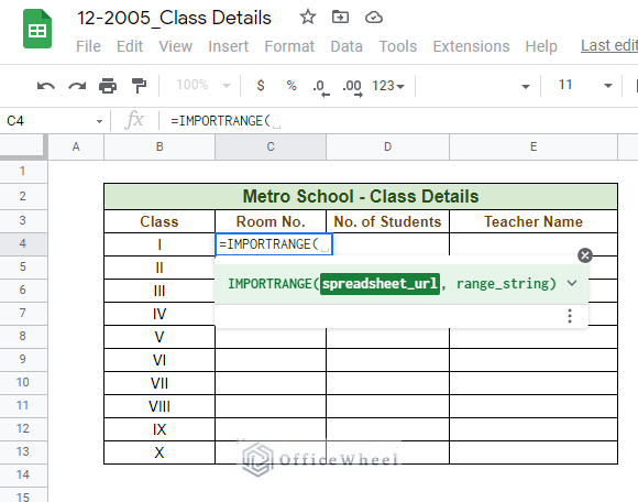
Step 1: Select the cell where you want to extract the data to. In our case, it is cell C4. Now, type =IMPORTRANGE(. This should open the prompt.

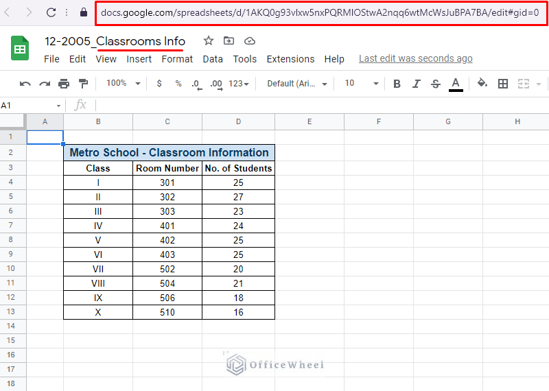
Step 2: Copy the URL from the other spreadsheet, Classroom Info in our case.

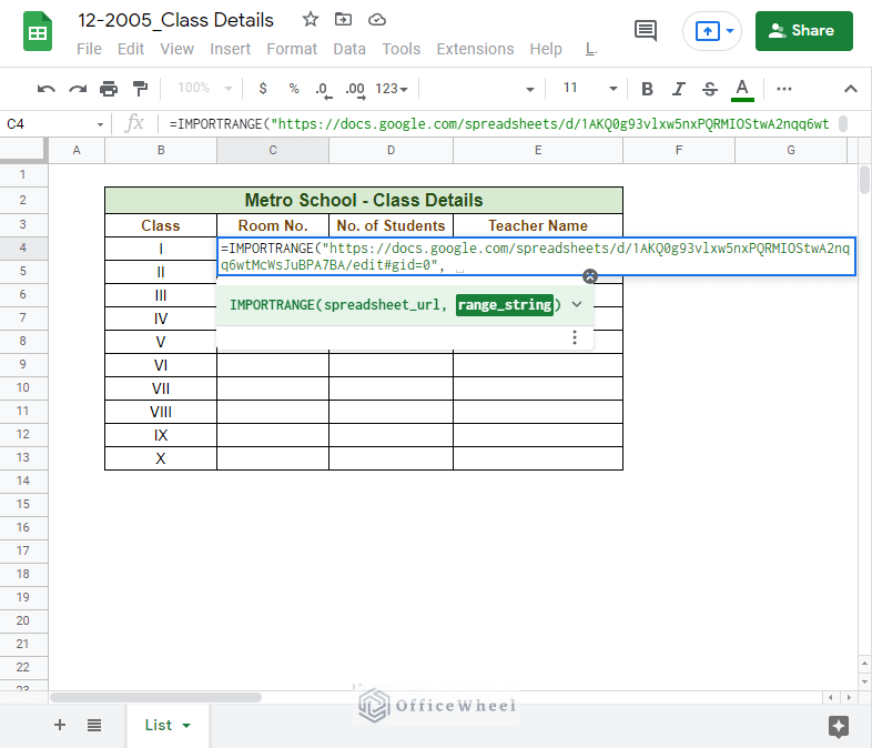
Step 3: In the place of spreadsheet_url, paste the copied URL within quotation marks (“”). Press comma (,) and move to the next part of the function.

Step 4: Note down the worksheet name and the range of cells where you are looking to extract the data from the other workbook.

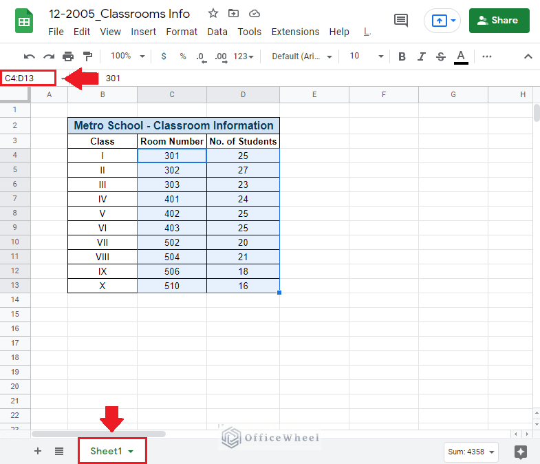
Step 5: Replace the range_string section concerning the worksheet name and the range within quotation marks. In our case, it is “Sheet1!C4:D13”.

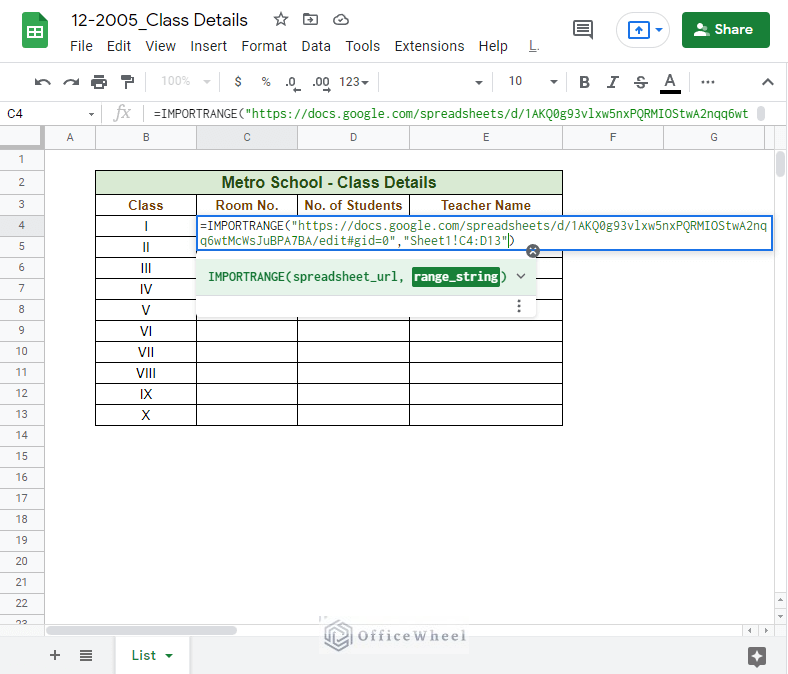
Step 6: Close parentheses and press ENTER.

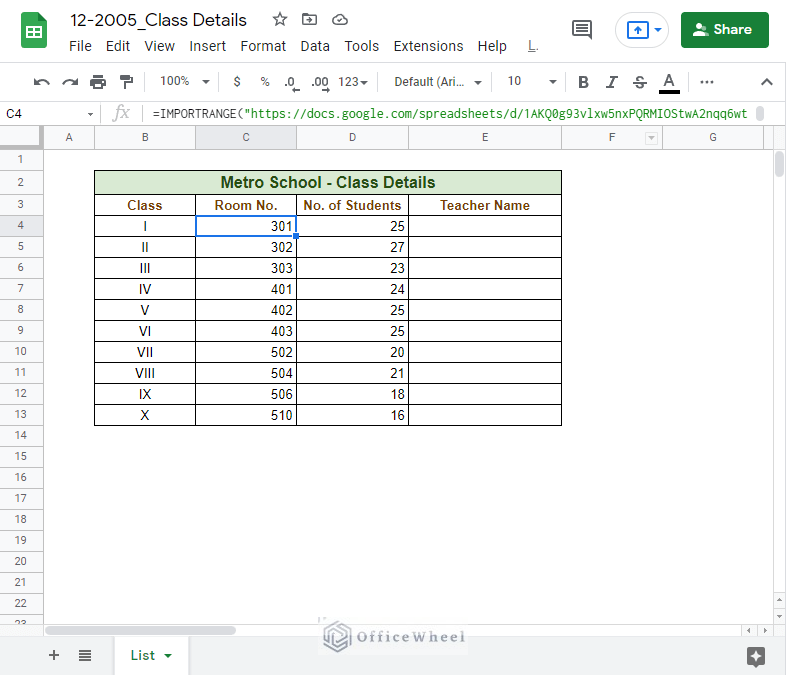
Great! We have successfully extracted two columns of data from another workbook.

Note: The IMPORTRANGE function is fully dynamic, this means that if we change any of the values of the cells in the extracted range, the values of the main workbook will also change.

For the remaining blank column, we will be extracting the data from a different workbook called Class Teachers. On top of that, we will take this chance to make a change to our input method for the spreadsheet_url field.

Read More: Reference Another Sheet in Google Sheets (4 Easy Ways)

Alternative: Using the Spreadsheet Key

In the previous extraction, we have copied and pasted the whole URL of the other Google Sheets workbook in the spreadsheet_url field. This time we will be pasting in its place the spreadsheet key of the other workbook.

Let’s see how it’s done.

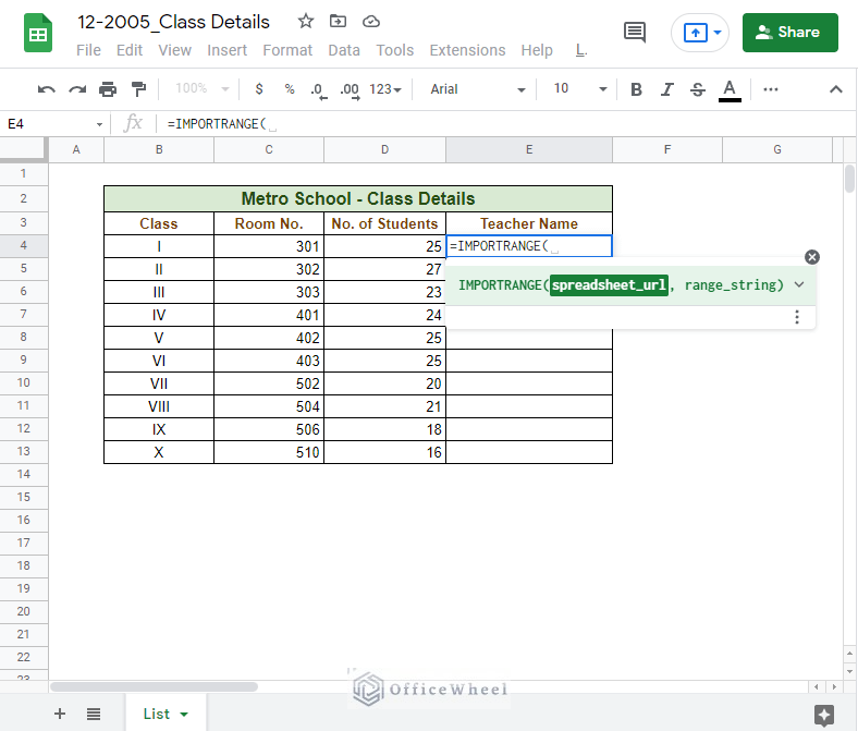
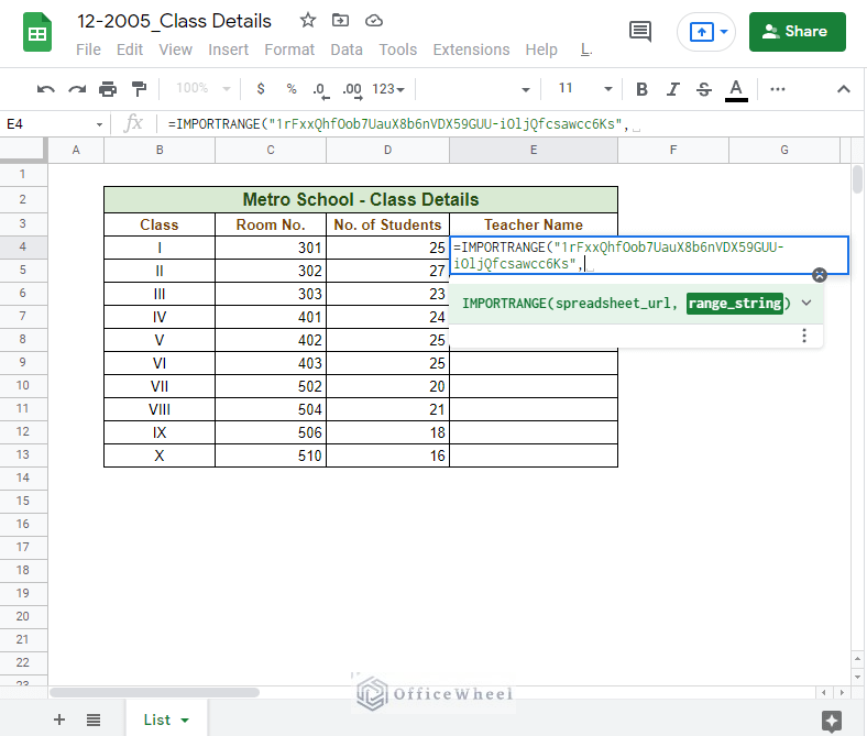
Step 1: Select the cell where you want to extract the data, cell E4 in our case, and type =IMPORTRANGE(.

Step 2: Copy the spreadsheet key from the other workbook. The spreadsheet key is a special string in the URL, like the one in the image below.

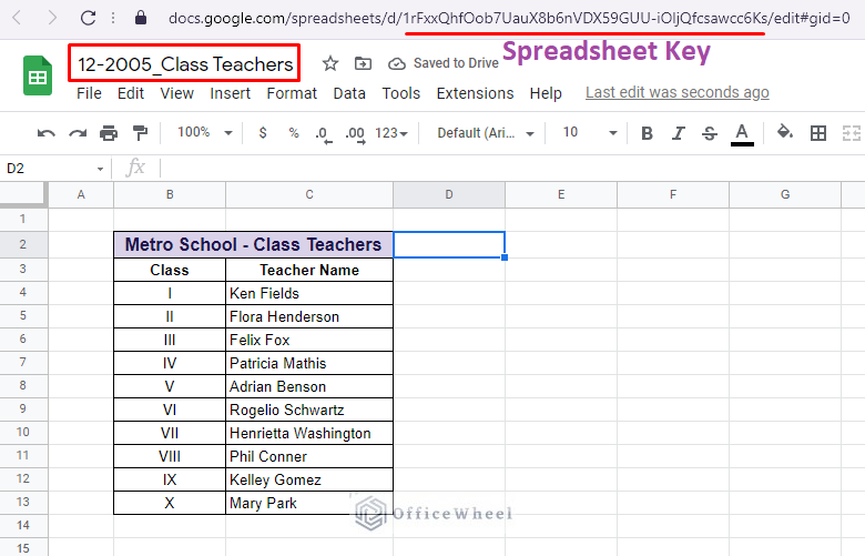
Step 3: Copy the spreadsheet key and paste it into the spreadsheet_url field. Remember to enclose the key in quotation marks! Press comma (,) to move to the next field.

Step 4: Note down the range of cells and the worksheet name from the other workbook.

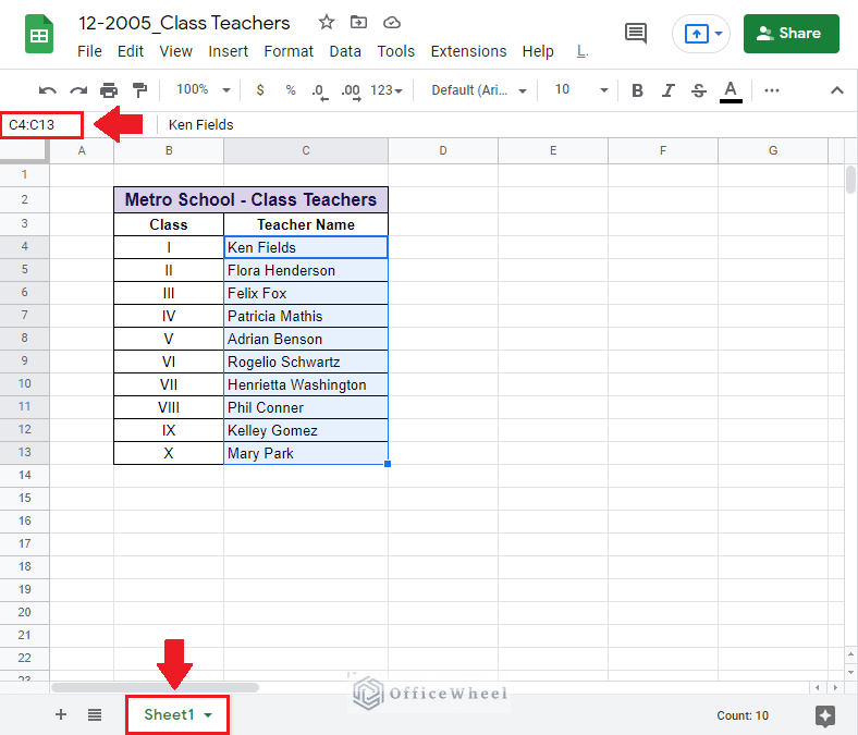
Step 5: Type in the reference worksheet name and cell range enclosed in quotation marks in the range_string field. Ours is “Sheet1!C4:C13”.

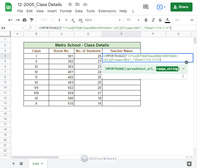
Step 6: Close parentheses and press ENTER.

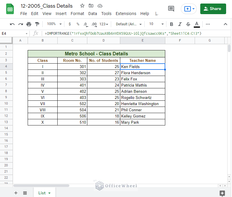
Similar Readings

• Reference Cell in Another Sheet in Google Sheets (3 Ways)
• Reference Another Tab in Google Sheets (2 Examples)

Clean Up Data

For our finishing touches, let us clean up our cell references a bit.

If you want, you can store the URL in-page and refer these cells into your IMPORTRANGE function:

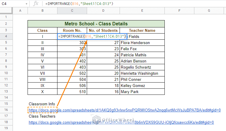
Referencing Classroom Info workbook

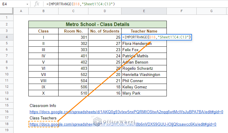
Referencing Class Teachers workbook

When directly referencing cells, you do not need to add quotation marks (“”).

Limitations

The IMPORTRANGE function currently has a limit of 50 cross-workbook links. But there is word that this might change soon.

Final Words

We hope that the steps that we have discussed have clarified for you how to reference another workbook in Google Sheets, which is mainly incorporating a simple yet versatile function, IMPORTRANGE.

If you have any questions or advice for us, please feel to comment.

Related Articles

• Pull Data From Another Sheet Based on Criteria in Google Sheets (3 Ways)
• How to Query Cell Reference in Google Sheets
• Dynamic Cell Reference in Google Sheets (Easy Examples)
• Lock Cell Reference in Google Sheets (3 Ways)
• Reference Another Tab in Google Sheets (2 Examples)
• Return Cell Reference in Google Sheets (4 Easy Ways)