The IFS Function in Google Sheets allows a user to test multiple conditions in a single formula. The formula may get too long but if you understand the conditions it takes, it is really easy to apply. This guide aims to discuss two important applications of the IFS function with multiple conditions.
A Sample of Practice Spreadsheet
You can download the datasets from the link below. After downloading you can practice on your own as we demonstrate here.
Introduction to IFS Function in Google Sheets
Objective
The objective of the IFS function is to verify whether one or more conditions are satisfied and returns a value that corresponds to the first TRUE condition.
Syntax
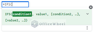
Inputs
- condition1: This is the first condition of the IFS The IFS function must have a minimum of one condition.
- value1: If condition1 holds TRUE then value1 is the output of the IFS function.
- [condition2, …]: These are the successive conditions. The IFS function stops evaluating further conditions whenever a condition holds TRUE.
- [value2, …]: These are the successive value of respective conditions. If a condition holds TRUE the IFS function returns the corresponding value.
Output
- The IFS function returns the value of the first TRUE condition.
2 Practical Examples of Using IFS Function in Google Sheets with Multiple Conditions
The first example of calculating student grades is the classic example of how the IFS function can be used. In this example, we calculate the student’s grades using the IFS function. The second example is a real-life application of the IFS function. Here, we can calculate sales commissions by providing conditions within the IFS function.
1. Calculate Students’ Grade
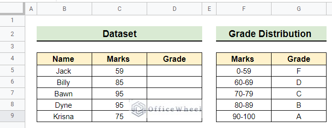
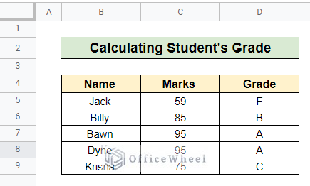
In our first example, the dataset contains a few students’ marks and their unknown grades along with a Grade Distribution for different ranges of marks. We are going to find the grades of the students using the IFS function with multiple conditions.
Steps:
- First, select the cell where you want to apply the IFS function. Here, we select cell D5.
=IFS(C5<60,"F",C5<70,"D",C5<80,"C",C5<90,"B",C5>90,"A")- After selecting the cell we write the above formula in the formula bar. It contains multiple conditions for finding the grade of the students based on grade distribution.
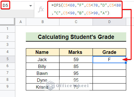
This formula returns the value of the first TURE condition which is “F” in this case.
- Finally, we use the fill handle and drag it down to find the grade of other students as follows.
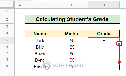
- At last, we got the grade of each and every student as you see in the following image.
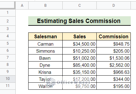
2. Estimate Sales Commission
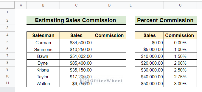
The following example involves the advanced application of the IFS function. Now, we want to estimate the sales commission of the salesman by putting multiple conditions within the IFS function in Google Sheets. For estimating the commission of a salesman, Percent Commission is given in our dataset. Here, we attach a picture of the dataset for your convenience.
Steps:
- Initially, we have to select the cell in which we want to apply the IFS function. In this instance, we select cell D5.
=IFS(C5<$F$5,$G$5,C5<$F$6,$G$6,C5<$F$7,$G$7,C5<$F$8,$G$8,C5<$F$9,$G$9,C5<$F$10,$G$10,C5<$F$11,$G$11,C5>$F$11,$G$11)*C5
- Then we put the above formula in the formula bar to get the commission amount for the first salesman.
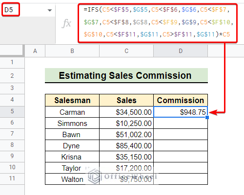
The return value of the IFS function is the value of the first condition that holds TRUE. Then, we multiply the return value with the cell C5 to calculate the commission.
- Finally, we use the fill handle and drag it down to estimate the sales commission for the other salesman like below.
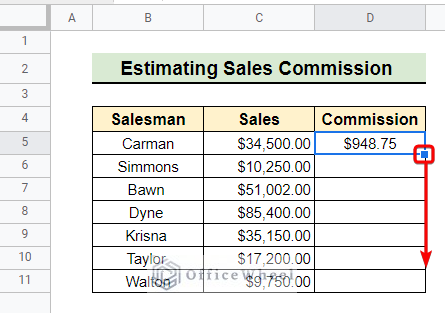
- Once we complete the fill handle operation we got the final result as follows.
Things to Remember
- The Nested IF Function can also employ for the above task. But the Nested IF function is long-winded than the simple IFS function. Basically, the IFS function obviates the Nested IF function of Google Sheets in some cases.
- The VLOOKUP Function can also be used here. It doesn’t require you to state every condition specifically as in the case of the IFS function.
- The IFS function needs cells to be static and dynamic simultaneously in its argument. So be careful about that when you write the formula in the formula bar.
- Click the bottom of the formula bar and drag it down to make the formula bar bigger. So that you can easily find if you made any glitch within the conditions of the IFS function.
Conclusion
I hope you have fully understood the IFS function with multiple conditions in Google Sheets with these two ideal examples. Further, If you have any questions regarding this article feel free to comment below and I will try to reach out to you soon. Visit our website OfficeWheel for the most useful articles.