Access and collaboration are two of the main driving forces behind Google Sheets and the other applications in the line.
As easy as it can be to share your worksheets over the internet via Google Sheets, we may also have to focus on the security of our data. And sometimes, simple sharing restrictions are just not enough.
Thus, it brings us to our topic today, how to lock cells in Google Sheets.
This brings us to the question:
When & Why is Locking Cells Necessary?
- You are sharing your workbook with a large audience. Many workbooks are shared publicly but leaving it on view-only mode may not cut it for every situation. You may need certain sheets or certain cells of your workbook to be restricted from third-party edits.
- You may need other users to fill up “input” cells. A form for example, where the user may need to fill up certain fields that apply to them, but not change other important cells or fields that have crucial information in them.
- Specifically, to protect cells that have complex or important formulas. The same applies to references.
How to Lock Cells in Google Sheets (For Multiple Situations)
1. Lock Specific Or a Range of Cells In Google Sheets
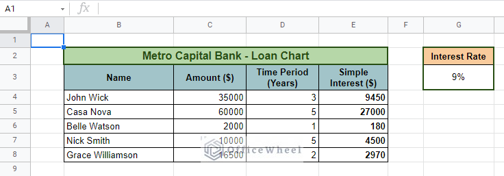
Our dataset today involves the calculation of the simple interest of certain clients of the Metro Capital Bank. Datasets like these usually have important calculation formulas and number constants that should not be changed.
This is a prime situation where cell locking is required, lest any of the executives mistakenly changes an important field while inputting data.
Lock Cells Step-By-Step
Step 1: Select a cell or a range of cells. In our case, we have chosen to lock the Interest Rate of our dataset, cells G2 and G3.
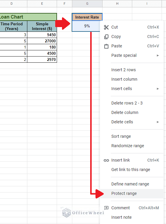
Step 2: Right-click over the selected cells. A drop-down menu will appear.
Step 3: Near the bottom of the menu, you will find the Protect range option. Click on it.
Step 4: The Protected sheets & ranges menu tray will appear on the right-hand side of the window.
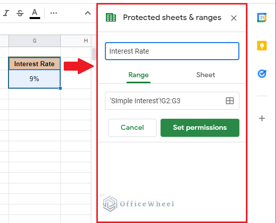
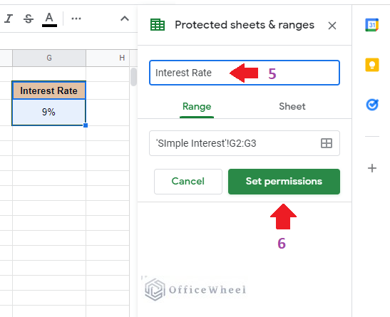
Step 5: We recommend that you name your selected range, for the sake of convenience. We have named our Interest Rate.
Step 6: Click on Set permissions to move on to the next step.
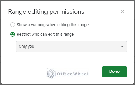
Step 7: For now, we will leave the presented options in the Range editing permissions window as it is (more on this will be discussed later in this article). Click Done.
You have successfully locked the range of cells from further editing!
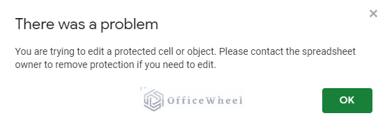
Now when someone else tries to edit these locked cells they will be hit with the following message:
An alternative to steps 2 and 3:
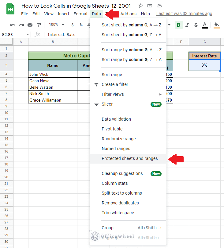
Another way to bring out the Protected sheets & ranges menu tray is by using the Data tab located on the top of the window. Here you will find the Protected sheets and ranges option near the bottom half.
Now that we have the basics out of the way, it is time to look at the certain conditions that we can add to this type of cell protection depending on various situations.
Read More: How to Protect Formulas in Google Sheets (2 Quick Ways)
2. How to Lock a Column in Google Sheets
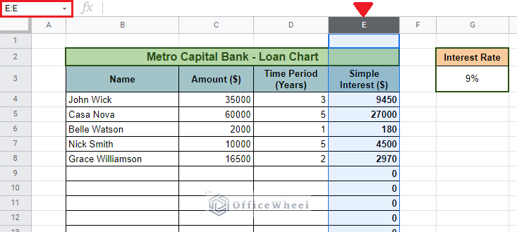
Let’s first take a look at how we can protect a particular column.
In our case, the Simple Interest column is the one that contains the formula, we don’t want anyone to mess with that.
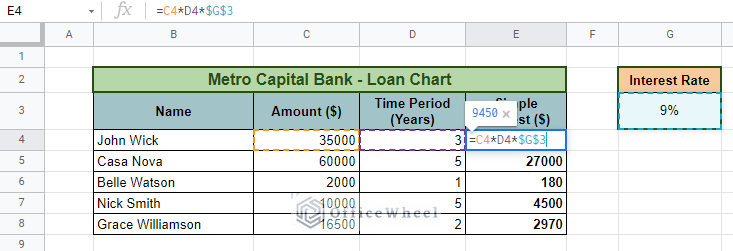
On top of that, it is highly unlikely that the rows of data will end at row 8. With every new customer, the number of rows will increase. Thus, it becomes crucial to lock the entire column, E, as we add more data to our table.
Having selected the column, we will open the Protected sheets & ranges panel as we showed in the previous section.
But now, focus on this section in particular:
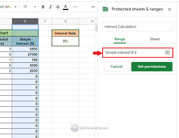
Here, Simple Interest is the name of the worksheet that we are currently on. The E:E represents the range of the selection.
Note: E:E describes that the entirety of column E has been selected. For performance’s sake, we can start our selection from cell E4 since that is where our formula starts from. The range will then become E4:E.
You can always change the range of your selection by clicking on the Select data range button:
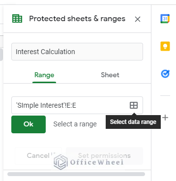
This will help you make direct selections within the worksheet. Click Ok when you are done.
All that remains now is clicking on Set Permissions > Done.
You have now successfully locked an entire column in your Google Sheet.
For a more in-depth guide, please read our How to Lock a Column in Google Sheets article.
Read More: How To Lock Rows In Google Sheets (2 Easy Ways)
3. Protect an Entire Sheet in Google Sheets
The need to protect the entire worksheet may arise more often than not.
Thankfully, Google Sheets presents us with this option in the same panel we have been working with so far, the Protected sheets & ranges option tray.
Here, to protect the entire worksheet, follow these steps:
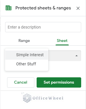
Step 1: Select the Sheets option in Protected Sheets & ranges.
Step 2: Click on the drop-down to open up the list of worksheets available in the workbook.
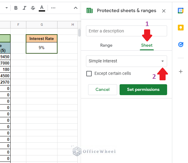
Step 3: Select your desired worksheet to be locked. We have selected our Simple Interest sheet.
Step 4: Set Permissions > Done
The worksheet is now successfully locked from further edits.
Note: Unfortunately, Google Sheets does not allow us to lock multiple worksheets at once. If you have to lock multiple worksheets, then you have to do so one by one.
Read More: Protect Range in Google Sheets (Easy Examples)
4. Lock an Entire Sheet Except for Specific Cells
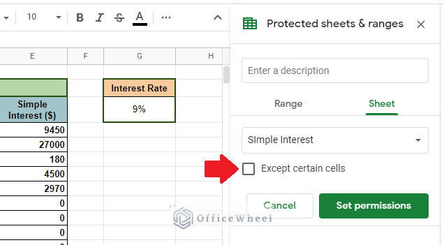
We will start this section from Step 3 of the previous section. We have the Protected sheets & ranges tray open and have our desired worksheet selected.
Now, to apply exceptions to our locked worksheet we must check the Except certain cells box:
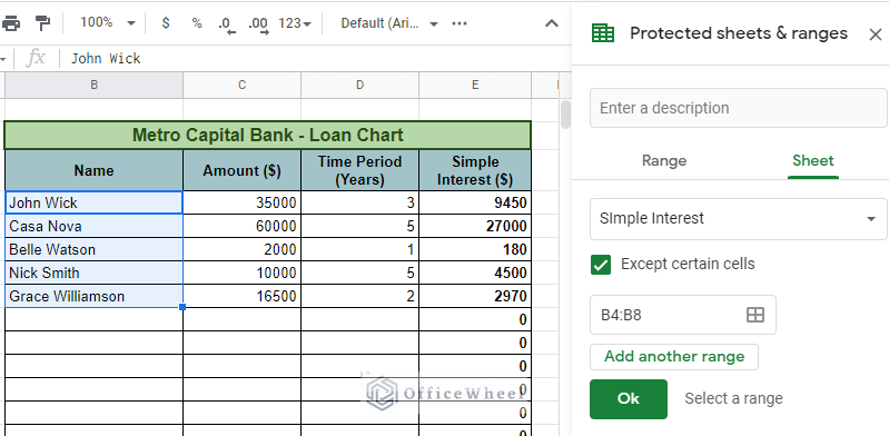
This will prompt you to add the range of cells that should not be locked in your worksheet.
Note: You can add more ranges for exception by clicking on the Add another range button:
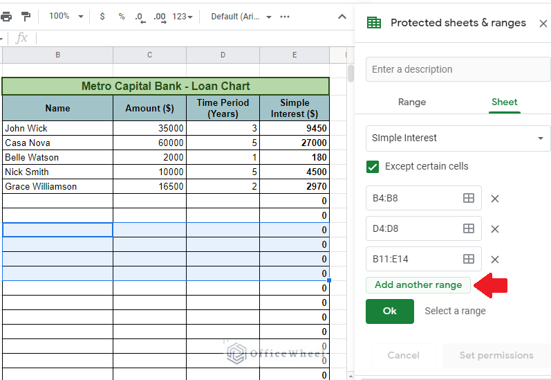
Click Ok and do the usual Set Permissions > Done process to finish up.
Read More: How to Lock Certain Cells in Google Sheets (With Quick Steps)
Collaborating With Others (Set Permissions)
The main agenda for locking cells in Google Sheets is for collaborating with others but to stop your collaborators from changing certain fields or sets of data. For that, Google Sheets allows us to customize how we will be presenting this protection to others in the share list.
We start at Step 6 of Section 1 and we can go about this in two ways:
- Give outright permission to Edit
- Give a soft warning when someone goes to Edit
Giving Permission
When everything is set in the Protected sheets & ranges panel, we will click on the Set Permissions button. As expected, the Range editing permissions pop-up will be presented.
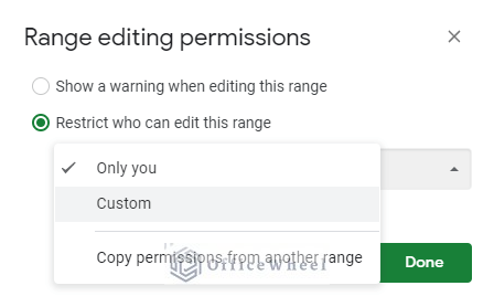
We will now select the drop-down menu and change from Only You to Custom.
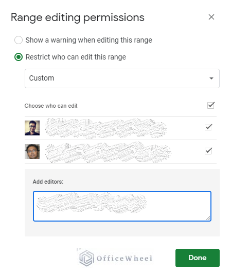
This will expand the window to show your initial collaborators and a section at the bottom where you can add the email addresses of other collaborators that you will permit to edit your workbook.
Giving Warning
Next up we have the soft edit warnings.
In the Range editing permissions window, we have the Show a warning when editing this range option.
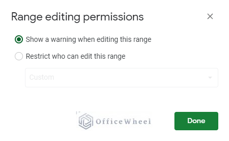
Checking this option will allow anyone to edit the worksheet, but it will always throw a pop-up warning every time someone wants to edit a restricted field.
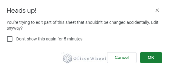
The warning pop-up looks like this:
In our opinion, this option is more of an annoyance and does very little in terms of protecting the worksheet.
Unlocking Cells in Google Sheets
Till now, we have talked about the various ways in which we can lock cells for security.
But what to do if we want to reverse these changes? How do we do it?
We can do this by following these four simple steps:
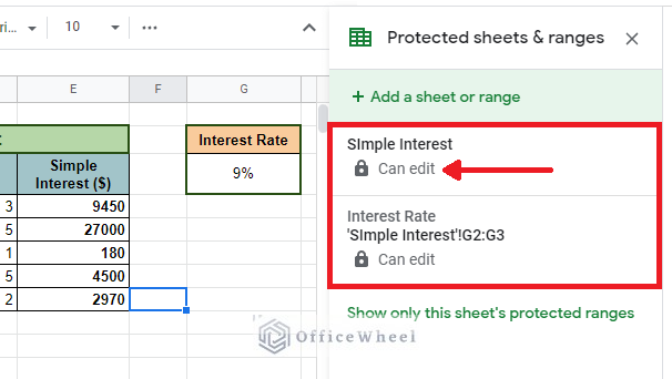
Step 1: Go to the Data tab and click on the Protected sheets and ranges option. This will open up the Protected sheets & ranges option tray.
Step 2: The Protected sheets & ranges option tray will show the list of locks and restrictions placed upon the workbook. If you are the creator or have permission to edit, the words Can edit will be shown under the name.
Step 3: Select the lock that you want to remove by double-clicking it. This will open up the edit menu.
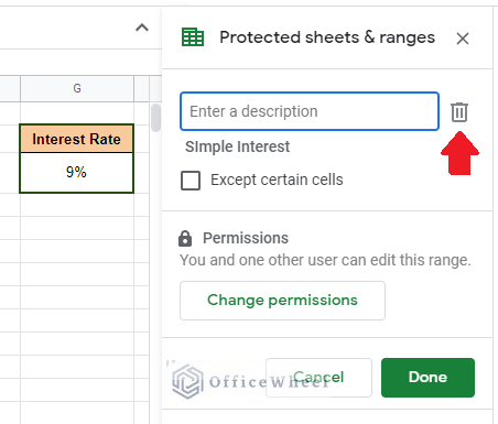
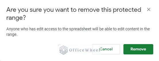
Step 4: Click on the Delete icon to remove the lock. You will be presented with a final warning pop-up to remove this lock. Click Remove.
Final Words
We hope that you have found the article informative. We have tried to cover all the different situations and iterations of how to lock cells in Google Sheets. The bottom line is that we must always remember not to neglect the security that comes with modern conveniences like Google Sheets.