[Fixed!] Wildcard Is Not Working in Google Sheets (5 Solutions)

In Google Sheets, we use wildcards to find data and perform different operations using functions. But sometimes problems arise that the wildcard is not working in Google Sheets. In this article, we will learn the possible reasons why wildcards do not work while used in functions and their solutions.

What Are Wildcard Characters in Google Sheets?

Wildcards are special types of characters that are used to represent characters in cells. There are mainly three wildcards that are used in Google Sheets to represent characters:

• An asterisk (*) is used to match any sequence of characters.
• The question mark (?) represents any single character.
• The tilde (~) is used before the wildcards to consider them as normal text.

5 Possible Reasons and Solutions If Wildcard Is Not Working in Google Sheets

We can use wildcards in different criteria-based functions like SUMIF, COUNIF, AVERAGEIF, and so on. In the following examples, we will briefly show you how to use the wildcards in these functions in Google Sheets. Then we will discuss the possible reasons and solutions if wildcard is not working in Google Sheets. So let’s start!

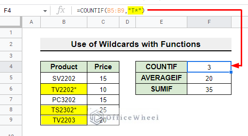
• Firstly, you can use an asterisk (*) in the COUNTIF function to match numbers and count them.

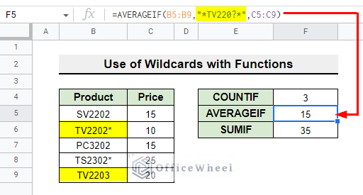
• Secondly, you can use the question mark (?) in the AVERAGEIF function to find values within the specified position and average them.

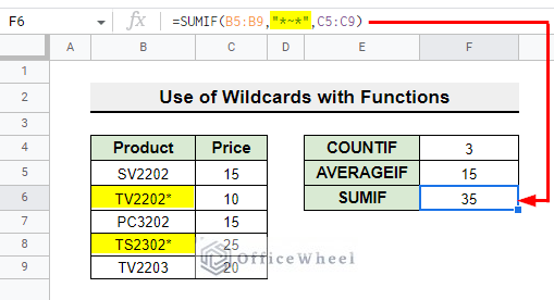
• Thirdly, you can use the tilde (~) to search values with wildcards and count them.

But, sometimes using these wildcards may not give you the expected results for various reasons. A discussion on the possible reasons why wildcards do not work in Google Sheets and their solutions with examples are given below.

Read More: How to Average If Cell Is Not Blank in Google Sheets (5 Ways)

Reason-01: Erroneous Cell Reference

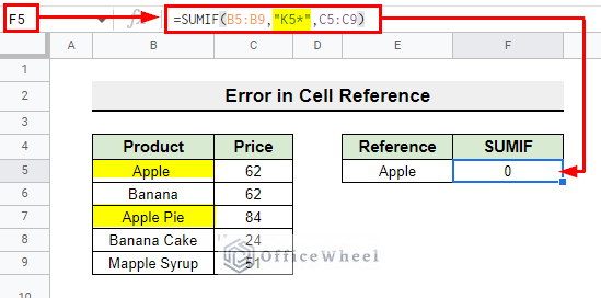
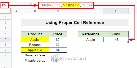
Assume you are using an asterisk (*) in the SUMIF function to add the price of an apple-made product. But the SUMIF function returns 0 instead of the total price.

• Use the wildcard asterisk (*) in this function to sum the price of the matching contents referenced by cell E5. However, the SUMIF function interpreted it as text rather than a cell reference because of the double quotation. That’s why it returned 0.

Read More: How to Use Wildcard with IF Condition in Google Sheets (3 Ways)

Solution: Using Proper Cell Reference

You can resolve this issue by using proper cell references. To do that-

• Use the ampersand (&) symbol in the function as shown below to keep the cell reference outside the double quotes.

Reason-02: Presence of Leading or Trailing Spaces

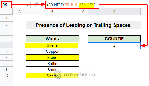
Now consider you are using the COUNTIF function to match words that start with S and end with E. But the function is returning 2 instead of 3.

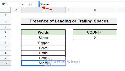
• In this case, we use the question mark (?) wildcard to search words that start with S and end with E.

• But the function is counting two cells instead of three cells. Here the problem is one cell contains leading space.

Solution: Removing Leading and Trailing Spaces

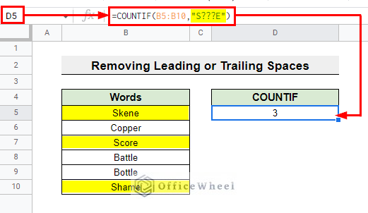
If there is any leading or trailing edge the COUNTIF function can not recognize the cell for the argument criteria. For that-

• You need to ensure that there are no leading or trailing edges existing in the cells. Then, the function will give proper results.

Reason-03: Uneven Use of Quotation Marks

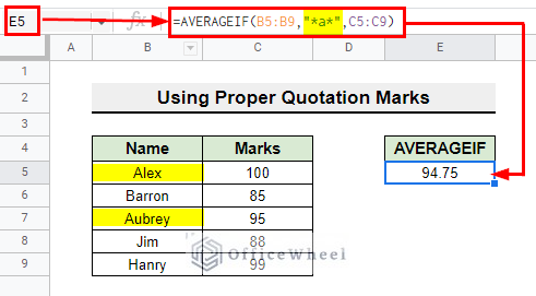
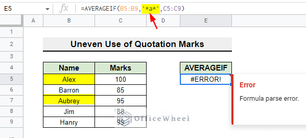
Assume you are using the AVERAGEIF function to calculate the average of the names that contain the letter A.

• For this case, use the asterisk (*) wildcard in the function to search names that contain the letter A and calculate the average.

• But the function will show an error rather than the average. Here, the problem is using a single quotation instead of a double quotation while declaring the criterion.
• You will also see errors if you use a double quote on one side and a single quote on another.

Read More: How to Average If Cells Have Multiple Conditions in Google Sheets

Solution: Using Proper Quotation Mark

The criteria argument for any function should be in double quotes. To solve the issue-

• You have to input wildcards in double quotation while inputting the criteria in the case of every criteria-based function.

Read More: How to Find Average in Google Sheets (8 Easy Ways)

Reason-04: Unusability of Wildcard with Dates

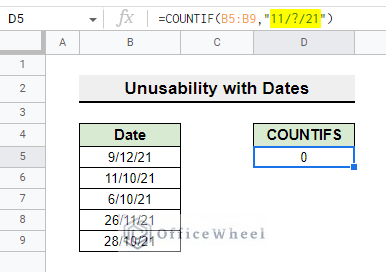
Furthermore assume that you are using the COUNTIF function to count the dates that are in October. But the function is returning 0 in place of 3.

• While using the wildcard question mark (?) in the function COUNTIF, the function returns an improper answer.

Solution: Using COUNTIFS and DATE Functions

Here the DATE function should be used in the criteria argument to declare the dates. For that-

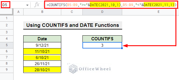
• You can use the DATE function along with the COUNTIFS function to get the proper output.

Reason-05: Using Improper Wildcards

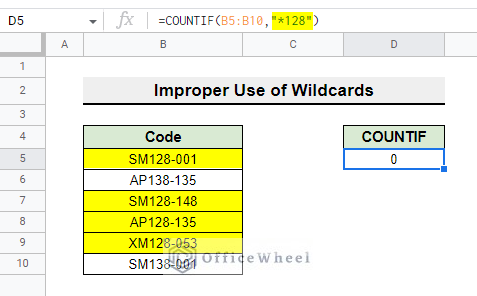
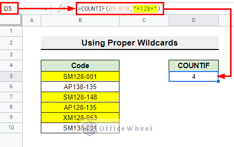
Suppose you are using the following formula to count the cells that contain the number 128 within the text using the COUNTIF function. The function is returning 0 in place of 4.

Solution: Using Proper Wildcards

To find numbers within texts you have to enclose the number within a double quotation and double asterisks (*). This is also applicable while you are searching within numbers. For that-

• Use the following formula-

Things to Remember

• Make sure that the range you are searching for is correct.
• Check that you are using the correct search function and criteria argument.

Conclusion

In this article, we have tried to cover the possible reasons why wildcard is not working in Google Sheets. Hopefully, this will help you to find your mistakes while using wildcards in Google sheets. Feel free to drop your query and suggestions in the comment section below regarding the article. For more Google Sheets-related articles you can visit our site OfficeWheel.

Related Articles

• How to Use Filter with Wildcard in Google Sheets (3 Examples)
• How to Use QUERY Function with Wildcard in Google Sheets
• Find and Replace with Wildcard in Google Sheets
• How to Average in Google Sheets If Value Is Not 0 (2 Simple Ways)