In terms of efficiency and reliability, knowing how to use Google Sheets average if multiple conditions exist is beneficial. AVERAGEIF, like all IF functions, will only compute values in a spreadsheet if certain conditions are met. AVERAGEIFS, on the other hand, allows you to check many criteria while AVERAGEIF just allows you to check for one.
A Sample of Practice Spreadsheet
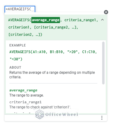
The AVERAGEIFS Function in Google Sheets
Understanding how to determine the mean or average number is crucial for daily living. It gives us an idea of where the center value is located in a dataset. It will be incredibly simple to work with any dataset if you know how to use the AVERAGEIFS function in Google Sheets.
Syntax:
5 Examples to Average If Cells Have Multiple Conditions in Google Sheets
There are primarily 5 possibilities, depending on the data and requirements. The example below illustrates each.
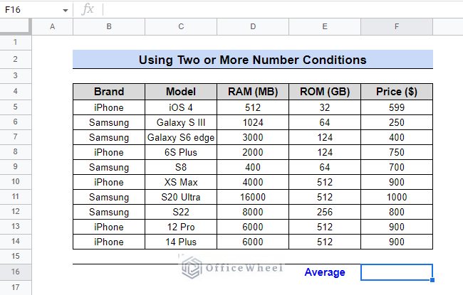
1. Using Two or More Number Conditions
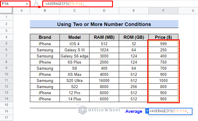
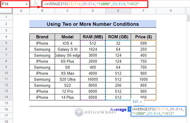
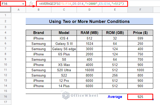
Assume we have data on the market price and specifications of Apple and Samsung, the top two mobile phone manufacturers in the USA. We’ll calculate the average cost of smartphones with 512 GB of ROM and more than 2000 MB of RAM.
Steps:
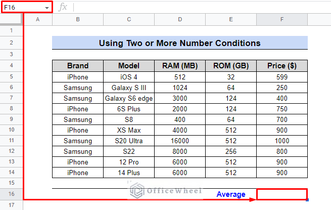
- We will select cell F16 to show the average.
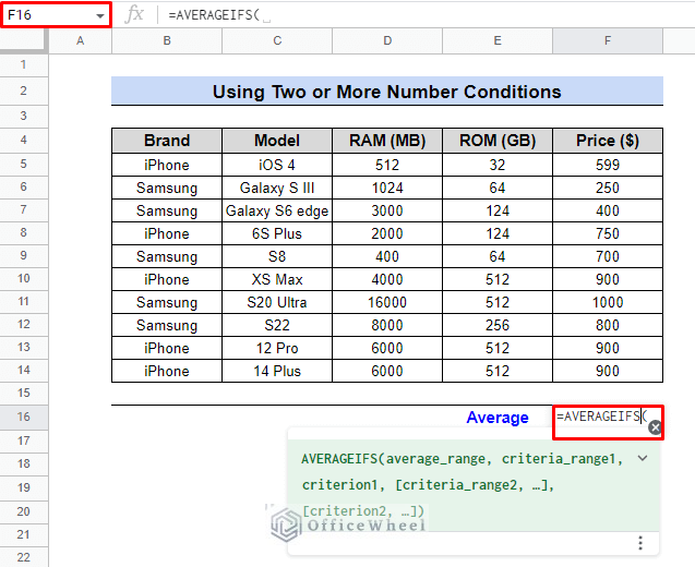
- Type =AVERAGEIFS to open parentheses in the formula box.
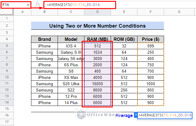
- We will select the cell range F5:F14 to calculate the average using a comma at the end.
- Now for searching for the first criteria, select the range D5:D14 followed by a comma.
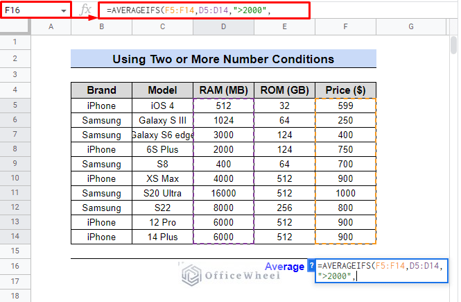
- Type “>2000” as criterion1 to check up on the range mentioned before.
- For the criteria_range2, select the range E5:E14. Don’t forget to put a comma at the end.
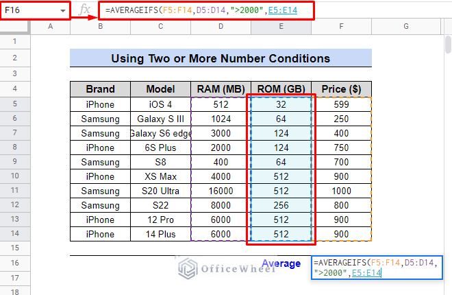
- Type “=512” as the second condition to check up on the ROM column.
- Final Formula:
=AVERAGEIFS(F5:F14,D5:D14,">2000",E5:E14,"=512")- Press ENTER to see the result.
Formula Explanation:
- F5:F14 is the range to calculate the average value.
- D5:D14 is the range of 1st criteria.
- “>2000” is the first condition within a quotation mark.
- E5:E14 is the second range of the second condition that we want to apply.
- “=512” is the second condition from the ROM column to checkup.
Technically 4 devices satisfy the requirements. Using the formula, the average cost of a smartphone is thus $925.
Read More: How to Find Average in Google Sheets (8 Easy Ways)
2. Applying Number and Text Conditions
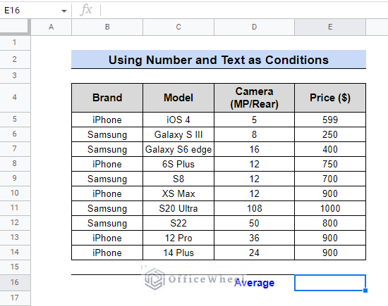
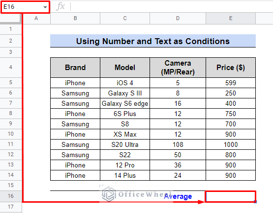
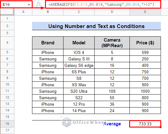
Once more, we have information regarding the price and camera characteristics of the two most popular US smartphone manufacturers. Assume we will discover the typical cost of Samsung smartphones with a rear camera that is more than 12 MP.
Steps:
- Go to cell E16.
- Use the following Formula:
=AVERAGEIFS(E5:E14,B5:B14,"Samsung",D5:D14,">12")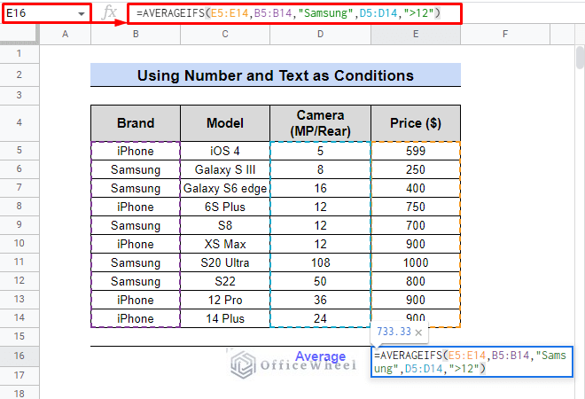
- Finally, click ENTER to obtain the average cost that fulfills the criteria.
Formula Explanation:
- E5:E14 is the range to calculate the average price.
- B5:B14 is the range of criteria_range1,
- “Samsung” is the first condition as a text value within a quotation mark.
- D5:D14 is the second range of criteria_range2,
- “>12” is criterion2 as second condition.
If you analyze the data, you’ll see that 4 Samsung devices feature rear cameras of 12 MP or greater. In this case, the average cost is $733.33.
Read More: How to Use AVERAGEIFS Function Between Two Times in Google Sheets
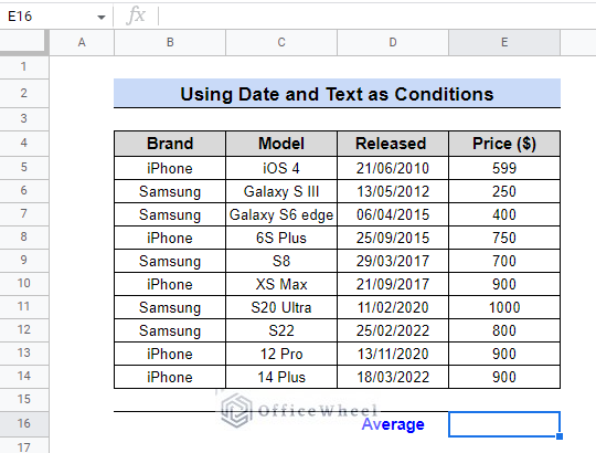
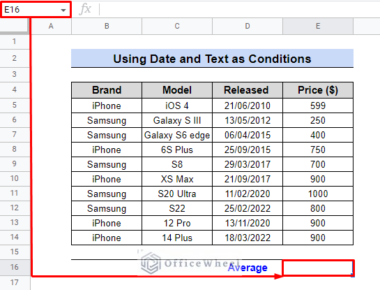
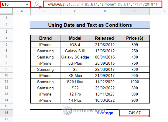
3. Utilizing Date and Text Conditions
You won’t always find the same type of data while doing google sheets average if multiple conditions related problems. Dates are a unique variation of the number. This example will show how to deal with a date and a text value as part of a conditional statement. Assume that our goal is to determine the average cost of iPhones from before 2018-more specifically, 1/1/2018.
Steps:
- First select cell E16.
- We will use the following formula to calculate the average cost.
Formula:
=AVERAGEIFS(E5:E14,B5:B14,"iPhone",D5:D14,"<1/1/2018")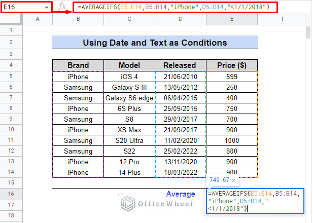
- Press ENTER to see the result.
Formula Explanation:
- E5:E14 is the range to calculate the average price.
- B5:B14 is the range for the first criterion.
- “iPhone” is the criterion as a text value for matching in the range.
- D5:D14 is the second range for the second criterion.
- “<1/1/2018” is the second condition as a date.
There are three iPhone devices from earlier than 2018 in the database. The three smartphones cost a total of $2249, with an average price of $749.67. Even with large datasets, we can solve it swiftly using the AVERAGEIFS formula.
Read More: How to Average in Google Sheets If Value Is Not 0 (2 Simple Ways)
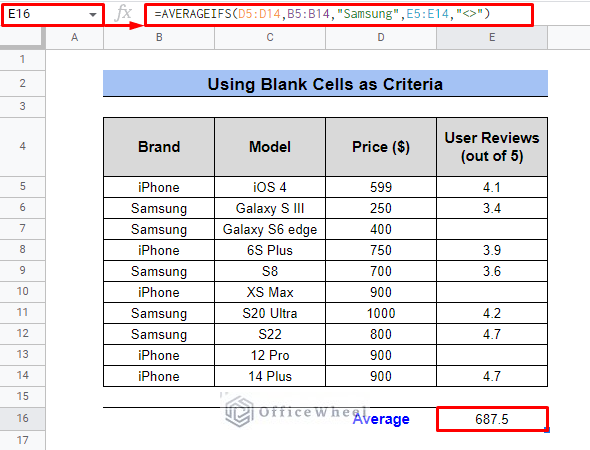
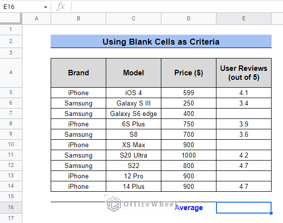
4. Using Blank Cells as Criteria
Imagine that we have a dataset that lists the user reviews (out of 5) and costs for both Apple and Samsung devices in this scenario. The cells are blank since not all of the models have real customer reviews. We’re looking for the average cost of Samsung smartphones without blank cells in user reviews.

Steps:
- First select cell E16 just beside cell D16 to show the Average.

- We will use the following formula to calculate the average cost.
Formula:
=AVERAGEIFS(D5:D14,B5:B14,"Samsung",E5:E14,"<>")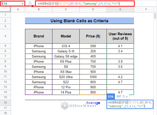
- To retrieve the result, press ENTER after closing the bracket.
Formula Explanation:
- For the average_range Type D5:D14.
- Select range B5:B14 for the first condition to look in.
- For this case, the first criterion is “Samsung” to match in the abovementioned range.
- Again, for Criteria_range2, type E5:E14.
- To identify non-blank cells type “<>” as the second condition.
You can see that there is just one Samsung device in the database that has a blank cell in the User Reviews (out of 5) column. Except for that one, there are four other devices. These four devices now cost, on average, 687.5 dollars.
Alternatively, we can also discover the average price of the iPhones that have missing data on User Reviews.
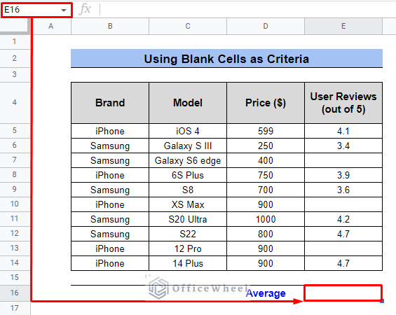
Steps:
- First select cell E16 to show the Average.
- Use the following Formula:
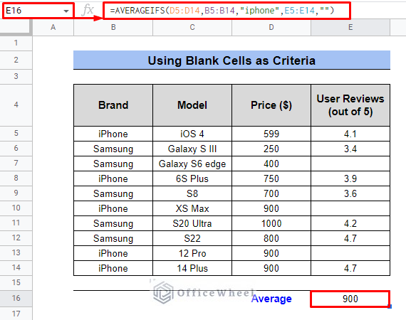
=AVERAGEIFS(D5:D14,B5:B14,"iPhone",E5:E14,"")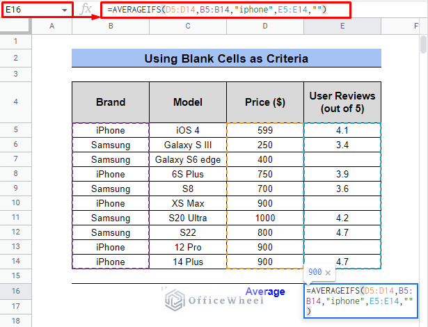
- Finally, press ENTER.
Formula Explanation:
- D5:D14 is the range to calculate the average price.
- B5:B14 is the range of criteria_range1,
- “iPhone” is the first condition as a text value.
- E5:E14 is the second range of criteria_range2,
- “” is criterion2 as the second condition that resembles blank cells.
The User Reviews column contains blank values for two iPhone devices. Thus, 900 is the combined average cost of these two devices.
Read More: How to Average If Cell Is Not Blank in Google Sheets (5 Ways)
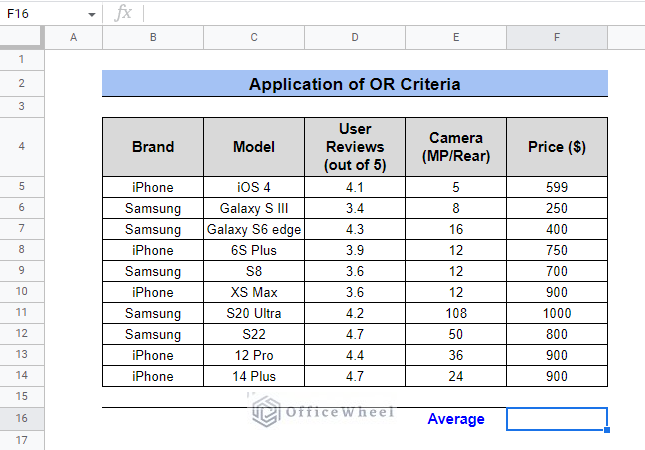
5. Implementing OR Criteria
Assume that You want to know the average price of Apple devices that have User reviews (out of 5) of more than 4.0 or Samsung smartphones that have a rear camera of more than 12 MP. Since we now have two independent criteria—either this or that—we must add two or more AVERAGEIFS in order to resolve the case.
Steps:
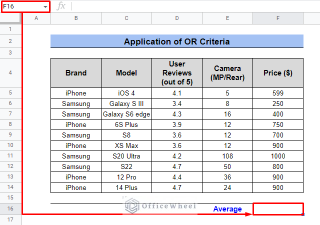
- We will select cell F16 to show the average.
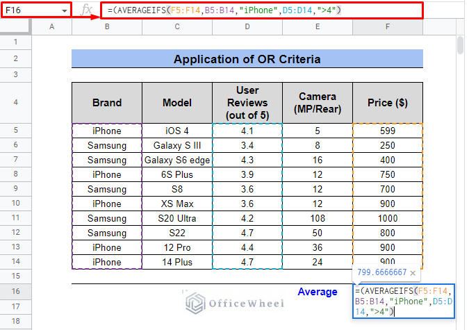
- We will write down the first condition of Apple devices that have User reviews (out of 5) of more than 4.0 using the following formula:
=(AVERAGEIFS(F5:F14,B5:B14,"iPhone",D5:D14,">4")
- To add the second condition in this particular instance, we utilize the operator “+“. The “+” operator functions as the OR operator.
- Afterward, type the following formula that fulfills the second condition of Samsung smartphones that have a rear camera of more than 12 MP
AVERAGEIFS(F5:F14,B5:B14,"samsung",E5:E14,">12")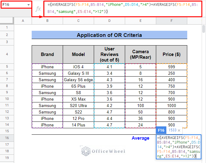
- To prevent mathematical errors, the entire formula is divided by two because there are two conditions with an OR between them.
- Final Formula:
=(AVERAGEIFS(F5:F14,B5:B14,"iPhone",D5:D14,">4")+AVERAGEIFS(F5:F14,B5:B14,"samsung",E5:E14,">12"))/2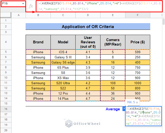
Three iPhones and three Samsung devices met the requirements. As a result, the average price is $766.5.
Read More: Use AVERAGEIFS with Multiple Criteria in Same Column in Google Sheets
Conclusion
You can add more conditions by repeating the process as much as you’d like now that you know how to work with multiple criteria, regardless of the type of data. Google Sheets functions like AVERAGE, and IF are very efficient while working with a large number of variables or multiple conditions. If you have any comments, please let us know. For more detailed information, please visit OfficeWheel.