How to Use the DATE function in Google Sheets (An Easy Guide)

In this simple tutorial, we take a deep dive into the DATE function of Google Sheets. We will discuss its importance and see a few of its uses as examples later in this article.

Let’s get started.

What is the DATE function of Google Sheets and how do we use it?

The DATE function is a great way to enter a date in Google Sheets regardless of date formatting.

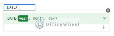
Many users may be confused or unsure of how to enter dates in Google Sheets since we have so many formats of dates we can use, and some of them may be invalid due to regional or other settings.

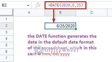
Since the DATE function simply takes the different aspects of a date, namely Days, Months, and Years, separately as arguments, and presents them in the default date format of the spreadsheet. Or, when used in other functions, as the correct date value.

To apply the DATE function to generate a date in the default format simply:

1. Open the function in a cell by typing =DATE(
2. Enter the respective values for year, month, and day separated by a comma.
3. Close parentheses and press ENTER to apply.

Why use the DATE function?

The primary reason to use the DATE function is to ensure that a date is entered and interpreted by Google Sheets correctly.

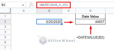
Many functions and formulas use dates and date values to produce results. Combining them with the DATE functions helps overcome any formatting issues that some date values might have. This is thanks to the DATE function outputting the correct numerical date value instead of a text format.

Furthermore, these combinations can be used to produce dates and date calculations in many different formats, which we will see later in this article.

Errors with DATE and How to Solve Them

1. The #N/A Error: The DATE function is commonly used to convert a different date format to the default one. However, you cannot simply apply or reference the date as an argument. If so, you’ll get a #N/A error.

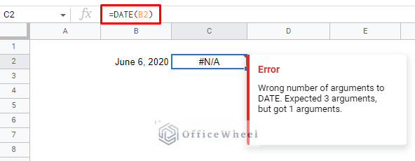
When trying to reference dates in the DATE function, you must combine it with other functions to fill the arguments (see example 2).

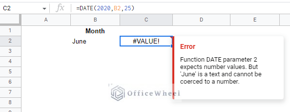
2. The #VALUE Error: The DATE function only accepts numerical values as its arguments. Text values will be considered invalid.

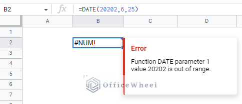
3. The #NUM Error: This error occurs when an invalid numerical argument is inputted. For example, a year value with 5 digits.

In the case of having more than 12 as a month value or having more days than the month actually has, the DATE function adjusts the value to the next valid date. For example, =DATE(2020,13,1) will return the value 1/1/2021.

Examples using the DATE Function in Google Sheets

1. Reference Date Values from a Different Cell

By now we know that the DATE function only accepts numerical values for its respective arguments. This also means that we can use cell references for these values to generate a date in the default format.

For example, here we have a dataset containing the Day, Month, and Year values:

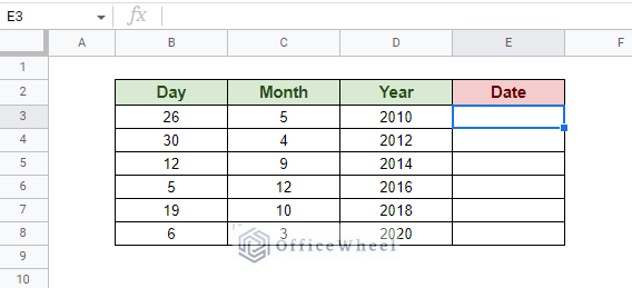
We can use this data to generate a date using the DATE function.

Simply open the DATE function in the Date column and fill the respective argument fields with the cell reference of the values. Close parentheses and press ENTER to apply.

Google Sheets will automatically suggest filling the column, or you can use the fill handle to apply the formula.

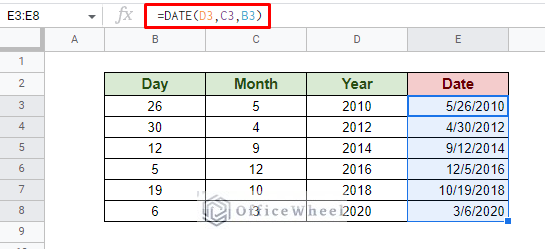
2. Use other Functions with DATE in Google Sheets

The best use of the DATE function is with other functions in Google Sheets. Let’s see two examples of this:

1. Formatting dates with the TEXT function.
2. Using other date functions of Google Sheets with DATE.

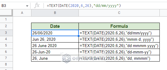
I. Using DATE and TEXT to Generate Different Date Formats

The TEXT function is a great way to convert a date to any format as a string in Google Sheets. As long as you know the text code for the date that is.

With the DATE function, we can input the valid date correctly in the TEXT function’s number field and then set the formatting.

Here are some examples:

II. Using Other Date Functions with DATE

In our first example, we’ve shown how we can use cell references to fill up the argument fields of the date function. And we have also tried to convert a text date to the default date format.

What if we combine the ideas?

Generate number arguments for DATE with a function and convert the date format.

Here we have a few dates that we want to convert to the default date format:

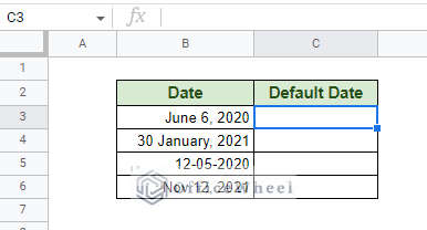
To fill the year, month, and day arguments we simply use the YEAR, MONTH, and DAY functions to extract the respective values from the date column. It will look something like this:

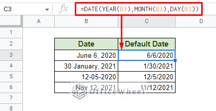
3. Add Days, Months, and Years to a Date Using the DATE Function

The fact that the DATE function has separate arguments for a year, month, and day can lead to another very important date calculation in Google Sheets. That is, adding days, months, and years to a date.

The application is quite simple, just add the number to the respective arguments.

For example, let’s say we want to add 10 days to a date. The date formula becomes:

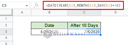
As you can see, adding 10 days to the date, 6/25/2020, has moved the date to the next month. The same will happen when adding months and years that cross over to the next value.

To add 7 months to the date:

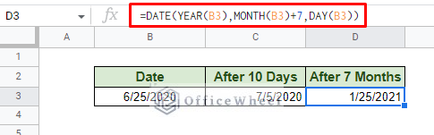
To add 3 years to the date:

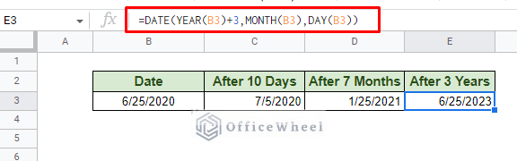
Learn More: How to Format Date with Formula in Google Sheets (3 Easy Ways)

4. Subtract Days, Months, and Years to a Date Using the DATE Function

Subtracting days, months, and years to a date with the DATE function is similar to adding these values. We simply subtract the respective values from the arguments.

Let’s see some examples.

First, subtract 30 days from the date:

Next, subtract 10 months from the date:

Finally, subtract 3 years from the date:

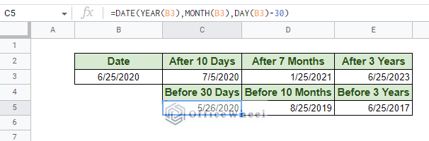
Final Words

The DATE function of Google Sheets is a great way to insert or use dates in the application. On its own, the function always returns the date in the default format, with other functions it returns the date value. Both of which are great uses.

Feel free to leave any queries or advice you might have for us in the comments section below.

Related Articles for Reading

• Add 7 Days to Date in Google Sheets (And More)
• Find if Date is Between Dates in Google Sheets (An Easy Guide)
• Calculate if Date is Before Today in Google Sheets
• Calculate if Date is After Today in Google Sheets
• How to Subtract Dates in Google Sheets (An Easy Guide)