We often need to know the specific amount of a particular type of number within a range. Like most schools publish their results not showing the marks but showing the grade points. And this grading system is usually classified like- 80~100% is equivalent to “A”, 70~79% is “B” etc. So it is important for them to calculate the number of total students with grades A, B, C or all. In this article, we have tried to demonstrate some easy methods on how to COUNTIF between two numbers in Google Sheets.
A Sample of Practice Spreadsheet
You can download the Google Sheets used to demonstrate methods in this article from here.
2 Easy Methods to Count Cells Between Two Numbers with COUNTIF Function in Google Sheets
Now let me show you two easy ways to COUNTIF between two numbers in Google Sheets.
1. Applying Single COUNTIF Function
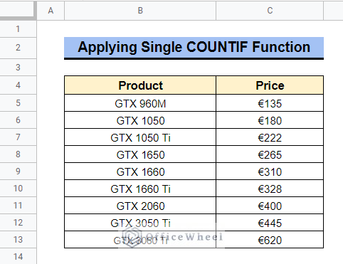
We have a dataset of products with their corresponding prices here. What we want is to count available products whose prices are greater than a specific value. Suppose, we want to count available products whose prices are greater than “€300”.
Steps:
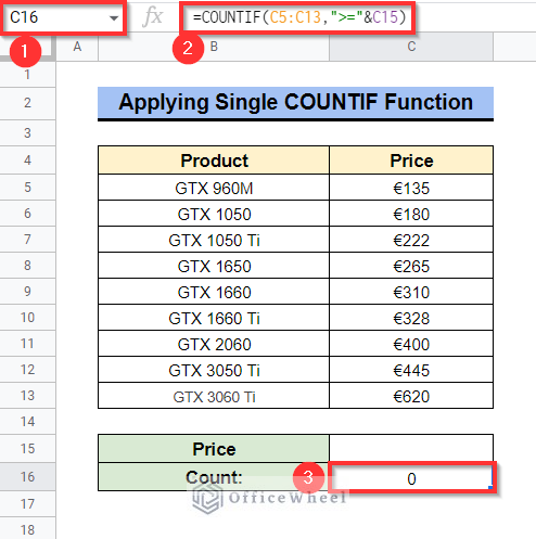
- In the following dataset, select Cell C16, apply the following formula and press Enter-
=COUNTIF(C5:C13,">="&C15)The output we will get is “0” as no such entry is in Cell C15.
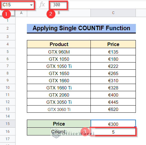
- Now, select Cell C15, type “300” and press Enter-
You can see that the total number of available products whose prices are greater than “€300” is “5”.
Read More: Difference Between COUNT and COUNTA in Google Sheets
2. Merging Multiple COUNTIF Functions
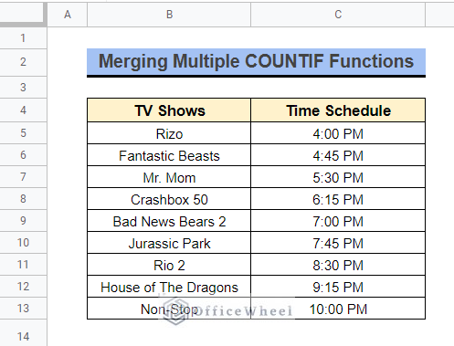
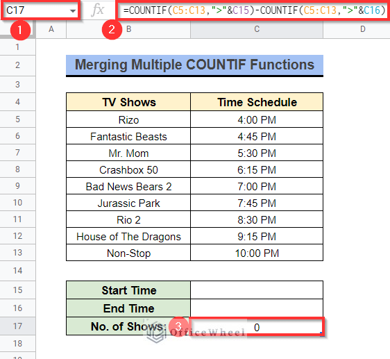
Suppose, we have a dataset of the Time Schedule of TV Shows on HBO. What we want to know is the number of TV shows within a specific time range. Let the time range be 4:30 PM to 8:00 PM.
Steps:
- In the following dataset, select Cell C17, apply the following formula, and press Enter-
=COUNTIF(C5:C13,">"&C15)-COUNTIF(C5:C13,">"&C16)We got the output as “0” as there are no such entries in Cell C15 and Cell C16.
Formula Breakdown
- COUNTIF(C5:C13,”>”&C15)
Here, the function counts the total number of available values that are greater than the time in Cell C15.
- COUNTIF(C5:C13,”>”&C16)
And here the function counts the total number of available values that are greater than the time in Cell C16.
- COUNTIF(C5:C13,”>”&C15)-COUNTIF(C5:C13,”>”&C16)
What this combination will do is 1st function result minus 2nd function result. And the difference will give us the number of shows between the times.
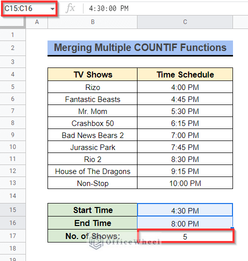
- Now, select Cell C15 then type “4:30 PM” and press Then in Cell C16 type “8:00 PM” and press Enter–
You can see that the output “No. of Shows” is “5”.
Read More: How to Calculate Hours Between Two Times in Google Sheets
4 Alternatives to Count Cells Between Two Numbers in Google Sheets
The COUNTIF function has limitations because it can’t deal with multiple criteria, so if we take the help of some other functions then there are a lot of ways to COUNTIF between two numbers in Google Sheets. Here, I’ll show you 4 useful alternatives among them.
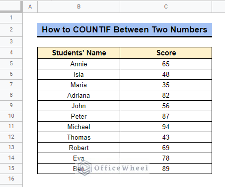
We will use the following sample dataset to describe these methods accurately. The dataset represents some students’ scores on a test.
1. Employing COUNTIFS Function
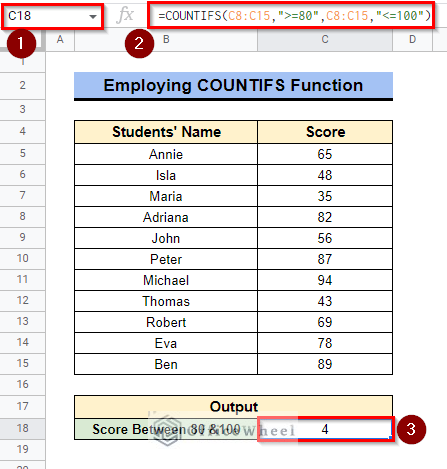
The COUNTIFS function returns the number of numeric values under multiple criteria. Like in the following example shown below, this function is used to meet two criteria, and which are to count numbers greater than or equal to 80 and less than or equal to 100.
Steps:
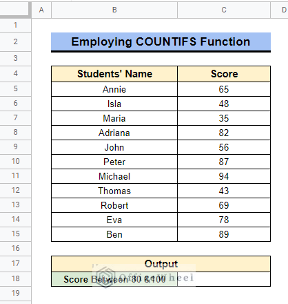
- Suppose, in the following dataset, we want to know the total number of students with scores between 80 and 100.
- Select Cell C18, apply the following formula and press Enter-
=COUNTIFS(C8:C15,">=80",C8:C15,"<=100")And soon after you will get the total number of counts like the image below.
Read More: How to Use IF Condition Between Two Numbers in Google Sheets
Similar Readings
- Generate Random Numbers or Text Between Limits in Google Sheets
- How to Find Correlation Between Two Columns in Google Sheets
- Insert Rows Between Other Rows in Google Sheets (4 Easy Ways)
- Calculate Number of Years Between Two Dates in Google Sheets
- How to Move Between Tabs in Google Sheets (3 Easy Ways)
2. Combining SUMPRODUCT and INT Functions
The INT function in Google Sheets finds the integer portion of numbers of a particular range of cells within a given criterion. The SUMPRODUCT function shows the result meeting all the criteria given in this function.
Steps:
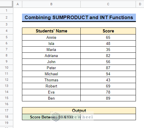
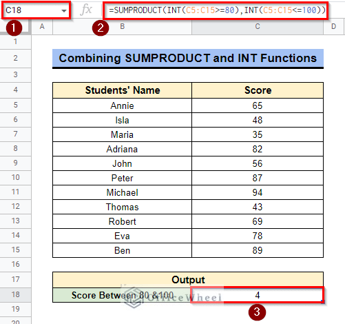
- Let’s assume, in the following dataset, we want to calculate the total number of students with scores 80 to 100.
- Select Cell C18, apply the following formula and press Enter–
=SUMPRODUCT(INT(C5:C15>=80),INT(C5:C15<=100))Then have a look, we got the same output as the previous method.
Formula Breakdown
- INT(C5:C15>=80),INT(C5:C15<=100)
As this function works under a single criterion, we have used this function twice, the first one working under a criterion that is finding numbers greater than or equal to 80 and the second one working under criterion that is finding numbers less than or equal to 100.
- SUMPRODUCT(INT(C5:C15>=80),INT(C5:C15<=100))
The SUMPRODUCT function then returns the total number of values that meets both of the criteria.
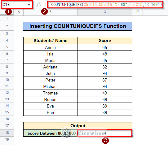
3. Inserting COUNTUNIQUEIFS Function
The COUNTUNIQUEIFS function returns the unique value of numbers based on multiple criteria.
Steps:
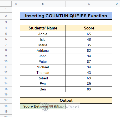
- Presume, in the below dataset, we want to get the total number of students with scores 80 to 100.
- Select Cell C18 and apply the following formula-
=COUNTUNIQUEIFS(C5:C15,C5:C15,">=80",C5:C15,"<=100")Here we can see that the result is showing “4” but the numbers between 80 and 100 are more than that. It’s because the function of the formula COUNTUNIQUEIFS is to return only unique values of the given criteria.
Read More: How to Find Unique Values Between 2 Columns in Google Sheets
4. Using Filter Option and Drop Down Menu
We can do the same without using any formula and using the built-in Filter option from the toolbar and the Drop Down menu that appears at the bottom right of the sheet after selecting a particular range of cells.
Steps:
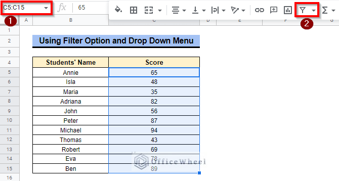
- In the following dataset, select Cell range C4:C15 and create a Filter function from the toolbar as follows-
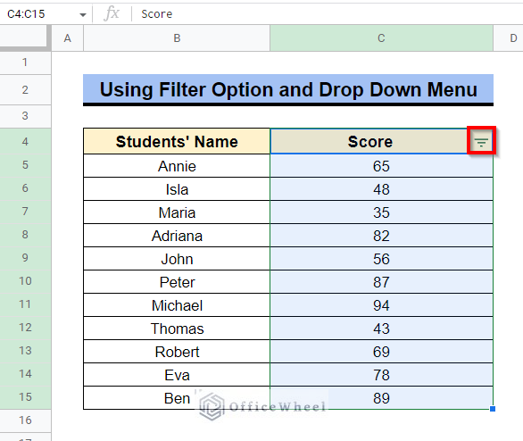
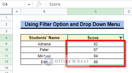
- Selecting that option, the Filter option will be created for that column from the first selected cell. Now, assume that we want to get all the values between 80 and 100. Press on the red-marked Filter Icon in Cell C4.
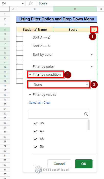
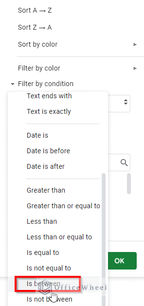
- A small window will pop up on your screen. Select Filter by condition and then the Condition box.
- Select Is between.
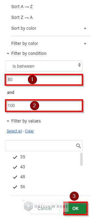
- Give input 80 in the first Value or Formula box and 100 in the second Value or Formula box and then select Ok.
- This will show only the values between 80 and 100.
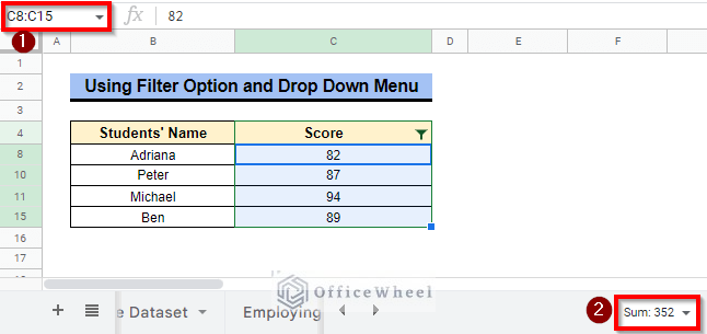
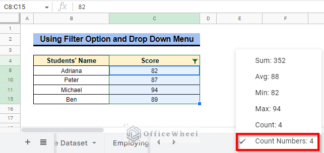
- Now select Cell range C8:C15 and then at the bottom right of the sheet select the Drop Down menu.
- At the Drop Down menu, you will find the total number of cells containing numbers between 80 and 100, and it is mentioned as Count Numbers.
Conclusion
We often need to classify based on numbers or scores and then comes the job to count the total numbers of each class. Meanwhile, in the following article, we have illustrated 4 easiest ways to COUNTIF between two numbers in Google Sheets. Hope this section will surely help you with your work. Visit our site officewheel.com to find more related articles that will help you to become more efficient and expert in Google Sheets.
Related Articles
- Find Number of Months Between Two Dates in Google Sheets
- How to Find Missing Values Between Two Columns in Google Sheets
- Conditional Formatting Between Two Values in Google Sheets
- Insert Lines Between Cells in Google Sheets
- How to SUMIF Between Two Dates in Google Sheets (3 Ways)
- Calculate Percentage Difference Between Two Numbers in Google Sheets
- How to Calculate Time Between Dates in Google Sheets (6 Ways)

