Filter with the AND Condition in Google Sheets (An Easy Guide)

When we filter for multiple conditions in a spreadsheet, we follow one of the two approaches to the relationship of the said conditions: AND or OR. In this article, we will specifically focus on how to filter with the AND condition in Google Sheets.

With the AND condition, the different conditions involved are dependent on each other.

Let’s see how it works.

Table of Contents

2 Ways to Filter with the AND Condition in Google Sheets

1. Use the Default FILTER Function Syntax to Filter with the AND Condition in Google Sheets

The FILTER function is a great way to filter data in Google Sheets. Not only does it leave the source data unchanged, but it also has all of the advantages of using a function in Google Sheets, like cell referencing or creating compound formulas with other functions.

The FILTER function syntax:

FILTER(range, condition1, [condition2, ...])

In this particular scenario, the FILTER function has another advantage. The default syntax of the function is naturally set to accommodate for the AND condition.

Notice the different condition fields that you can add in the function. Doing so will make these filter conditions dependent on each other. In other words, they will follow the AND condition.

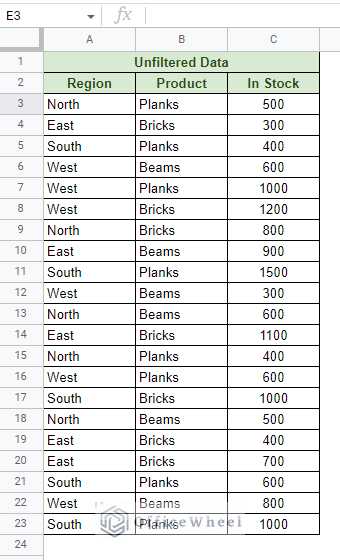
Let’s consider the following worksheet:

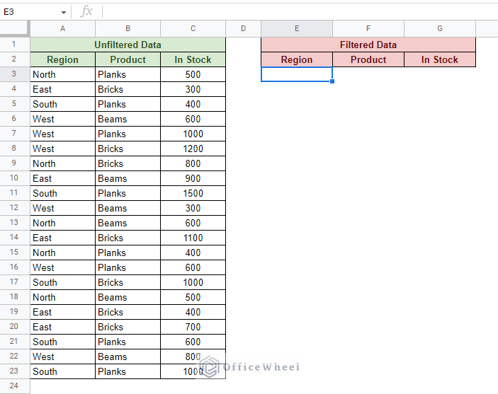
The best way to show the AND condition is to take a filter criterion from different columns. As such, let us try to filter all entries of the Product Beams that have more than 500 units In Stock.

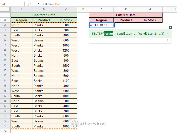
Step 1: Open the FILTER function and input the data range.

Step 2: Input the conditions for the filter.

To filter for “Beams” in the Product column:

B3:B23="Beams"

To filter for values above 500 in the In Stock column:

C3:C23>500

We will place each of these conditions separated by a comma (,). This represents the use of the AND condition.

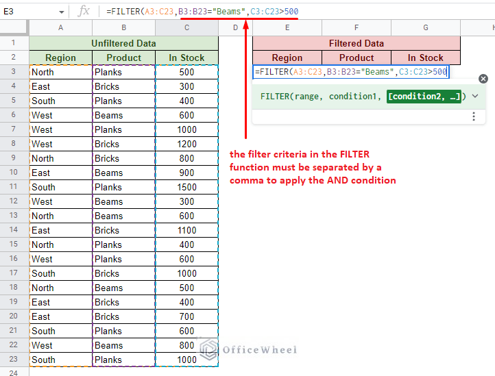
Step 3: Close parentheses and press ENTER.

=FILTER(A3:C23,B3:B23="Beams",C3:C23>500)

2. Use the Filter Feature of Google Sheets and Customize it to follow the AND Condition

Unless you mind any changes to the source data, the simplest way to filter with the AND condition over multiple columns in Google Sheets is by using the default filter.

This is a staple for any spreadsheet and generally, no complex formulas are involved, making this quite a beginner-friendly way to filter for basic conditions.

For this example, we will keep the filter conditions similar to the previous section: filter all entries of the Product Beams that have more than 500 units In Stock.

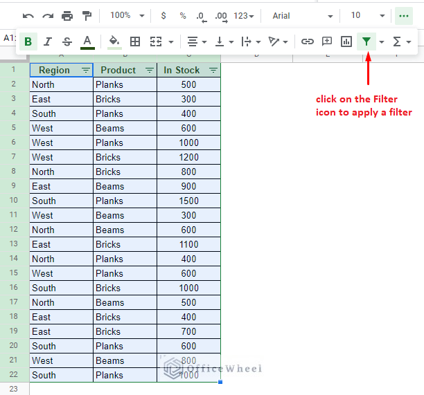
Step 1:Apply a filter over the source data. With the active cell placed in the source table or by highlighting the source data, click on the Filter icon from the toolbar.

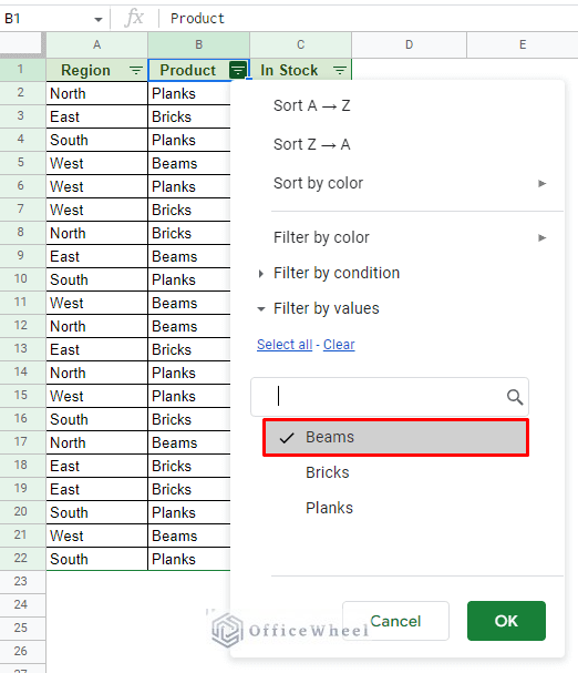
Step 2: Apply the first condition for the Product column. Select only “Beams” from the filter menu. Click OK to apply

Step 3: Apply the second condition from the In Stock column. Navigate to the Filter by condition section and select the Greater than option. Here, input 500.

Filter > Filter by condition > Greater than > 500

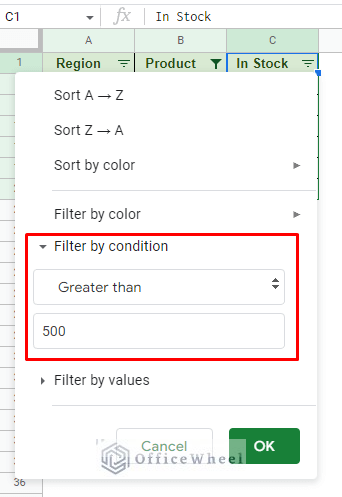
Click OK to apply.

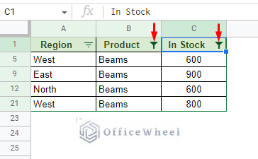
The final result:

Similar Readings

Combining the AND and OR Conditions to Filter Data in Google Sheets

Certain requirements may call users to apply both AND and OR filter conditions in Google Sheets.

For example, let’s say we want to filter for Bricks or Beams that have more than 500 units in stock.

In this case, the condition for the Product column will be in the OR condition (Bricks or Beams). And the condition for the In Stock column will be in the AND condition (more than 500).

Step 1: With the FILTER function open and the data range selected, we will apply the OR conditions first. The OR conditions will occupy only a single condition field of the FILTER function. It looks something like this:

(B3:B23="Bricks")+(B3:B23="Beams")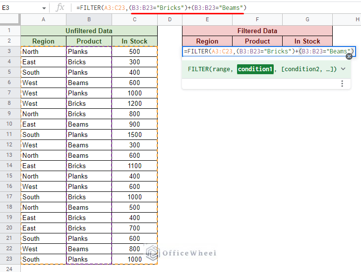

Step 2: Apply the AND condition next. Input a comma before adding the following condition:

C3:C23>500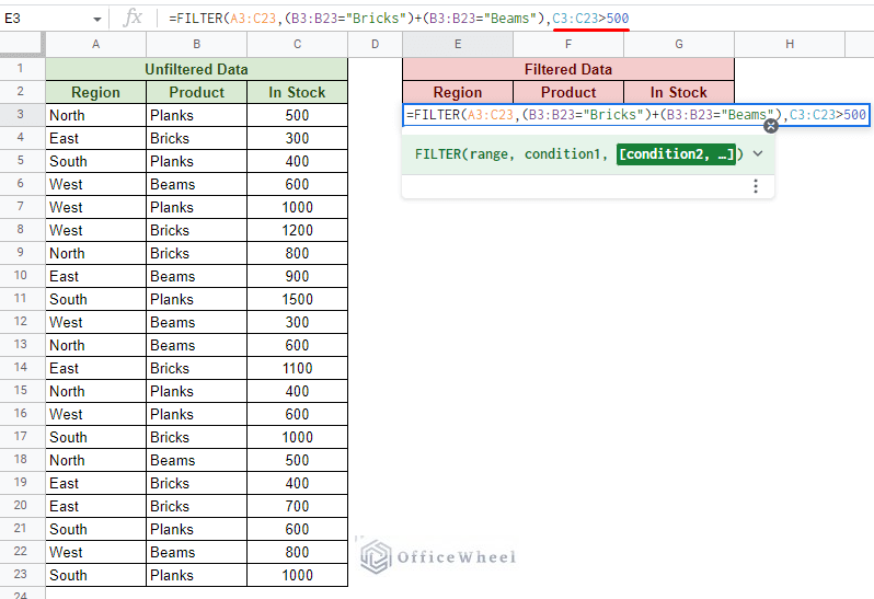

Step 3: Close parentheses and press ENTER.

=FILTER(A3:C23,(B3:B23="Bricks")+(B3:B23="Beams"),C3:C23>500)

How to Overcome the Error when there are no Results for the Filter

In the following image, you can see that we’ve tried to filter for Beams with more than 1000 units in stock.

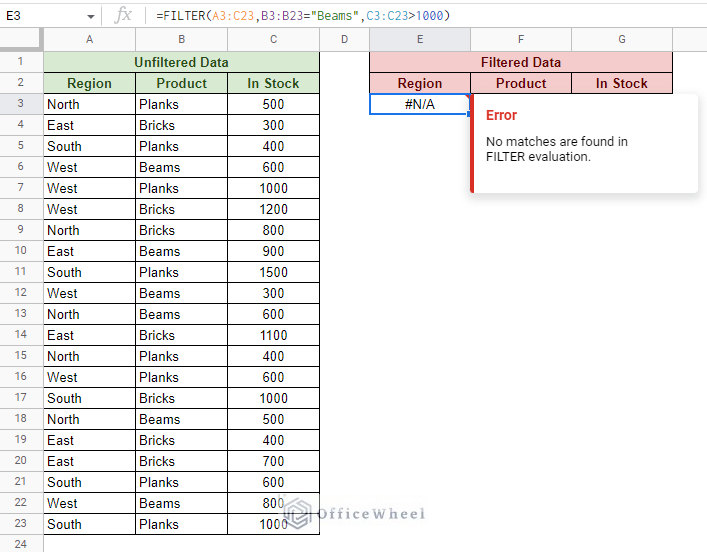
However, due to no entries being found that satisfy the conditions, we get an error.

This scenario is more common when we have to satisfy multiple conditions with the AND condition as the criteria are dependent on each other.

Thankfully, the solution for this problem is quite simple: enclose the FILTER formula inside the IFERROR function.

=IFERROR(FILTER(A3:C23,B3:B23="Beams",C3:C23>1000),"")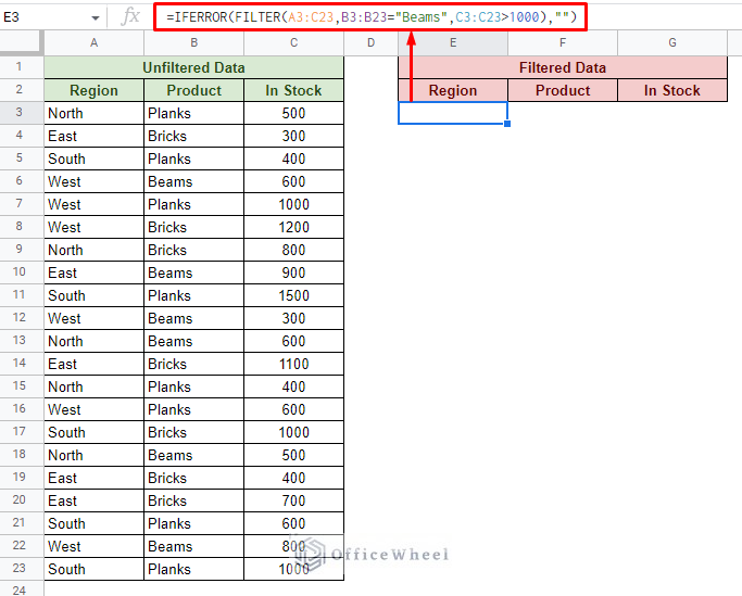

For the value_if_error field of the IFERROR function, we have asked the function to present a blank (“”).

Thus, it is a good practice to include the IFERROR function whenever you want to work with the FILTER function.

It is good to note that this error is not an issue when we use the default filter of Google Sheets.

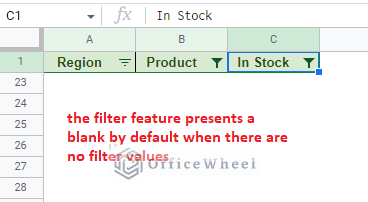
If no filter values are found, this filter naturally returns a blank, much like our result with the IFERROR.

Final Words

That concludes our simple guide to filtering with the AND condition in Google Sheets. We hope that the methods and tips we have shared with you come in handy in your Google spreadsheet tasks.

Feel free to leave any queries or advice you might have for us in the comments section below.