Today, we will look at how to pull data from an indirect range in Google Sheets. Just a disclaimer, this article focuses on cell ranges, not values of individual cells.
Let’s get started.
3 Ways to Use Indirect Range in Google Sheets
The core of our article today focuses on the INDIRECT function. While we may not dive into the function here, you can visit our Dynamic Cell Reference in Google Sheets article for a better breakdown of its capabilities with examples.
1. Locking Cell References for Indirect Range
Building on the idea of indirectly referencing cells in Google Sheets, we have our first practical use of using INDIRECT to reference range or ranges, that is to lock the starting and ending cell references of the range of cells we are going to use.
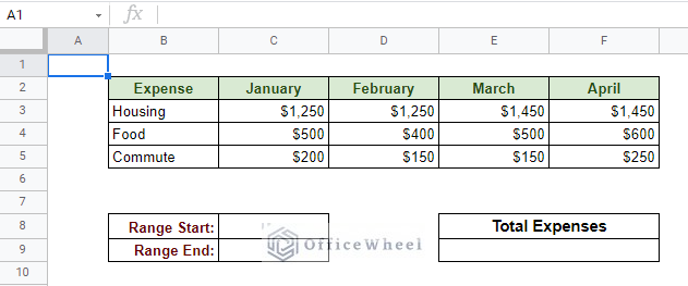
To show this example, we have the following worksheet:
Here, we have the costs incurred by certain expenses in each month. We have used the first four months of the year.
You will also notice the Range Start and Range End cells below the table. Here is where we will be designating the range of cells that we are going to calculate, and in this case, using the SUM function.
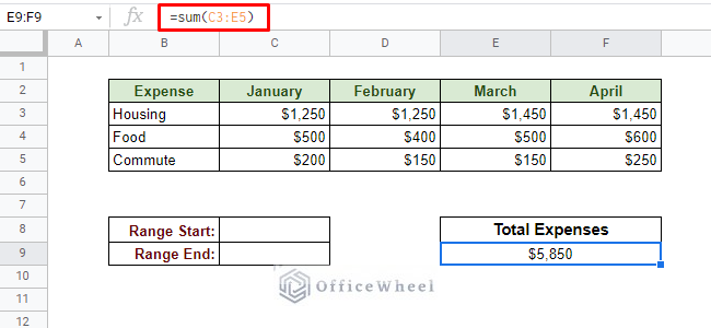
Let’s say we want to calculate the total expenses for the first three months of the year. We can simply do this by using the SUM function and the range of cells like so:
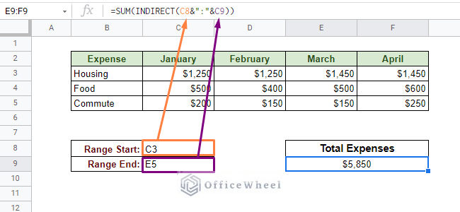
But, for the sake of extra security, we can designate the start and the end cells of the range separately in a different cell. Our formula will then incorporate the INDIRECT function to indirectly reference the new cell range.
=SUM(INDIRECT(C8&":"&C9))Formula Breakdown:
- INDIRECT(C8&”:”&C9): The indirect range reference away from the table. Helps to protect the formula cell from any changes.
- C8: References the starting cell of the range.
- &”:”&: The colon (:) defines the range in Google Sheets. It is concatenated by the ampersand (&) on both sides with the cell reference.
- C9: References the ending cell of the range.
- SUM: Sums the range indirectly defined by INDIRECT.
This type of formula works best when you have your formula cells secured but still want to make minor changes, especially to cell references indirectly.
Read More: Lock Cell Reference in Google Sheets (3 Ways)
2. Indirect Range from a Different Worksheet
Indirect range references are not confined to one worksheet. They can be retrieved from different worksheets in your spreadsheet.
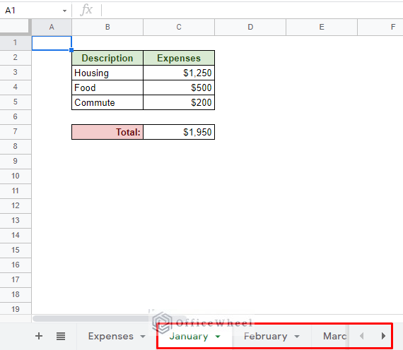
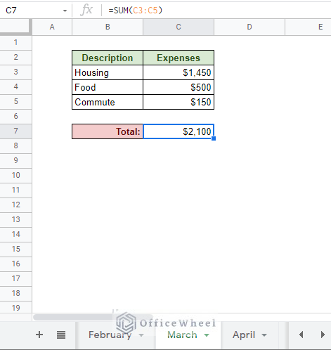
We continue from the last example of summing expenses of each month. This time, each month has its respective worksheet.
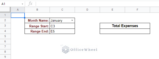
Our main worksheet, Expenses, now looks like this:
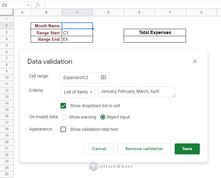
Note: You can apply the drop-down list in cell C2 by simply navigating to Data Validation from the Data tab (Data > Data Validation) and applying the following conditions:
We already know that to reference a range from another sheet we have to use the following format:
sheet_name!cell_rangeIn our case, it will be:
January!C3:C5
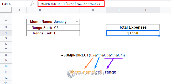
Now, using INDIRECT, our cell references will be:
- C2: Month Name
- C3: Range Start
- C4: Range End
Thus, our formula for the Total Expenses:
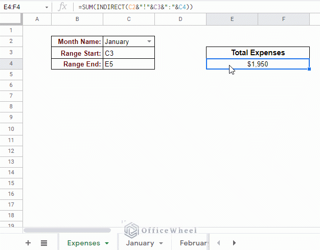
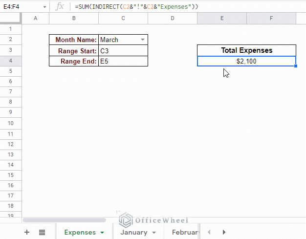
And thanks to the drop-down month list, we can calculate the expenses of each month.
With this method, not only is your formula cell protected, but you are also free to work with multiple sheets of your spreadsheet.
Read More: Reference Another Sheet in Google Sheets (4 Easy Ways)
Similar Readings
- Pull Data From Another Sheet Based on Criteria in Google Sheets (3 Ways)
- Google Sheets: Use Cell Value in a Formula (2 Ways)
3. Using Named Ranges to Indirectly Reference Cells
Another aspect of Google Sheets that the INDIRECT function takes advantage of is Named Ranges.
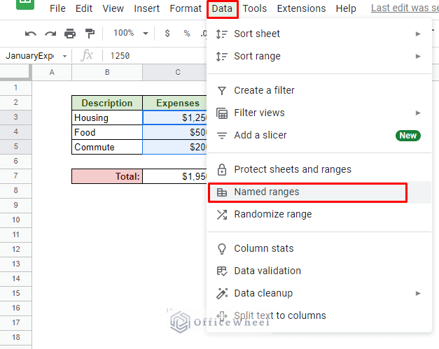
To apply a named range, you simply select the range of cells, navigate to Data > Named ranges option.
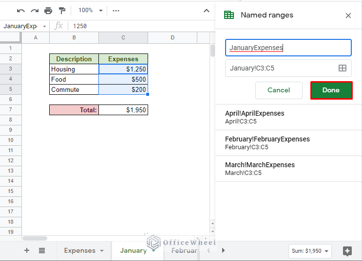
Next, you simply apply your desired name to the selected range and click Done. We have applied a Named Range for the Expenses column for each month.
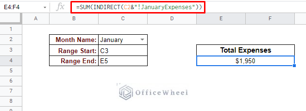
The fun part about named ranges is that you can pull this range from any worksheet. And taking advantage of that fact, we will apply it to our Expenses worksheet.
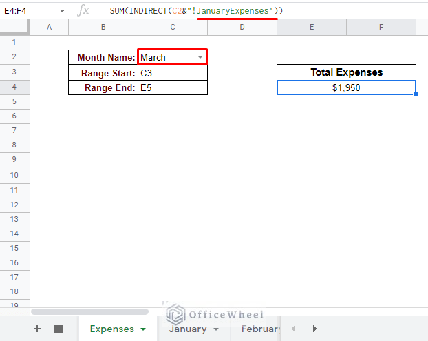
However, a limitation of this formula is the named range itself. Each named range is different. So, if we change the month name in the Expenses worksheet, we will get an error in value, as the named range given does not change.
The Total Expenses shown is still $1950 (January) whereas it was supposed to be $2100 for March.
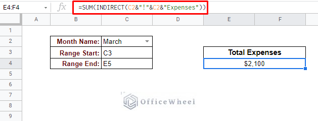
To remedy this problem, we must make some modifications to our formula. That is, making sure the month name also changes for the named range from the drop-down menu. Luckily for us, the named ranges were named according to their respective months, but also leaving the general naming convention intact for all of them.
=SUM(INDIRECT(C2&"!"&C2&"Expenses"))The new formula in action:
Note: Not only Named Ranges, but you can also use INDIRECT to indirectly refer to any range that is in the form of a string. For example, a cell may contain the string “C3:C5” and you can use INDIRECT to utilize this range. You can learn more about it in our Cell Reference From String in Google Sheets article.
Final Words
That concludes all the ways we can apply indirect range in Google Sheets from the same or different worksheets, or a different spreadsheet entirely. We hope that the three major methods we have discussed come in handy. Know that these are general examples, you can modify these methods and ideas to suit your needs.
Please feel free to leave any queries or advice you might have for us in the comments section below.
Related Articles
- Find Cell Reference in Google Sheets (2 Ways)
- Reference Cell in Another Sheet in Google Sheets (3 Ways)
- Variable Cell Reference in Google Sheets (3 Examples)
- Reference Another Tab in Google Sheets (2 Examples)
- How to Query Cell Reference in Google Sheets
- Dynamic Cell Reference in Google Sheets (Easy Examples)

