Today, we will look at how to use the Protect Range option in Google Sheets. We shall implement it for two scenarios: the first for a range of cells in a worksheet and the second to protect the entire worksheet.
Let’s get started.
How to Use Protect Range in Google Sheets
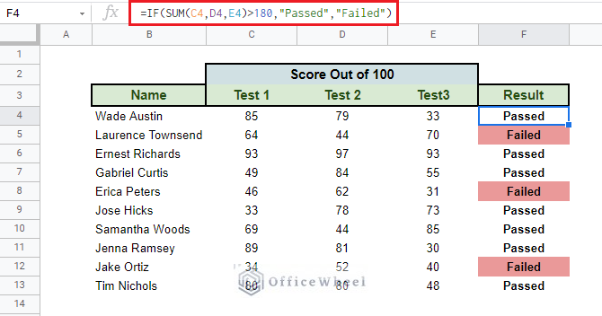
To show our process, we have the following dataset that has a Name, Scores, and a Result column that contains a formula.
1. Protect Selected Range in a Worksheet in Google Sheets
To apply Protect Range in Google Sheets, we must first select the range of cells that we want to protect and then navigate to the option.
Navigating to Protect Range for Selected Cells
We can go about two ways to reach the Protect Range menu.
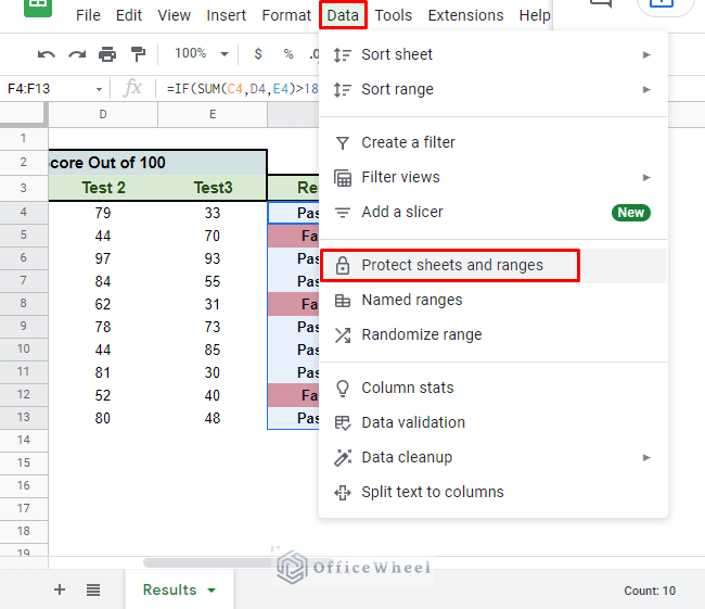
The first is from the Data tab. From the Data tab, select the Protect sheets and ranges option.
Data > Protect sheets and ranges
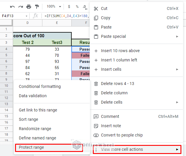
The second way is by right-clicking over the selected range. This should open a bunch of options. You have to navigate to the bottom to the option View more cell actions to find Protect range.
Right-Click > View more cell actions > Protect range
Read More: How to Lock a Column in Google Sheets (Simple Examples)
Applying Preliminary Conditions
The Protected sheets & ranges menu looks something like this:
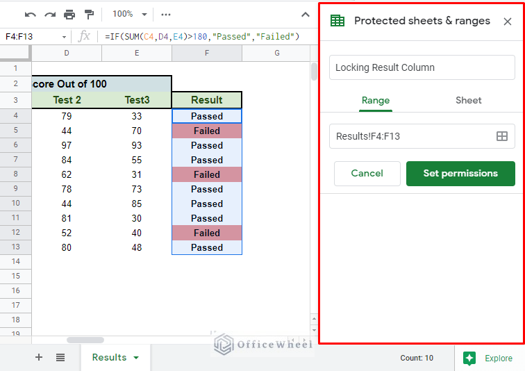
We have two sections to note here:
- The name section: You can name your protected range. Even though it is optional, it is always a good idea to do so.
- The range section: This section shows the range of selected cells that you are going to lock. You can also change the range from here.
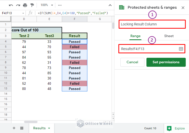
You will notice that in the second half of the menu, the Range section is selected. We will see the Sheet section later in this article.
If you are satisfied with the current conditions, click Set permissions to get into the meat of the protection.
Read More: How to Lock Certain Cells in Google Sheets (With Quick Steps)
Setting Permissions for the Protected Range
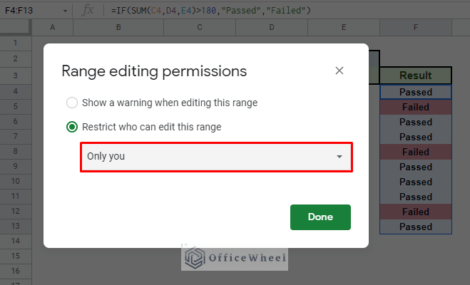
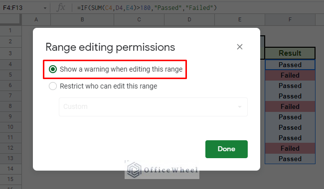
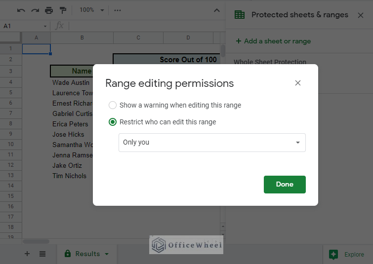
Here in the Range editing permissions, we are presented with three options.
- Only you: This option is presented to us by default. What this does is allow you, the owner, to be the only one able to edit the protected range.
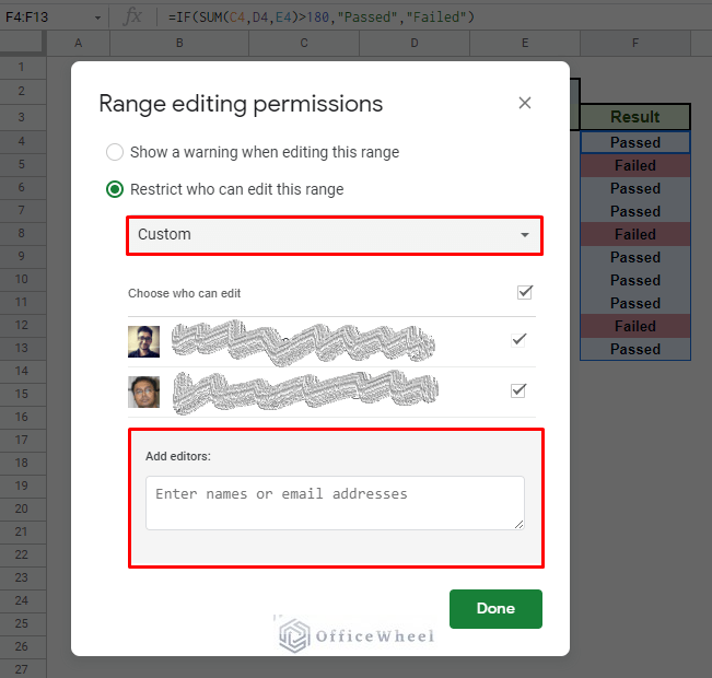
- Custom: Clicking on the drop-down will present you with the second option, Custom. This option allows you to add collaborators/editors for the locked range by entering their email addresses.
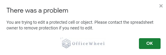
For these two conditions, if a third party tries to edit the locked range, they will be hit with the following message.
- Show a warning when editing range: This final option does not necessarily lock cells but presents us with a warning message whenever we edit the selected range. Making it the least secure of the permissions available but can work as a quick solution depending on the need.
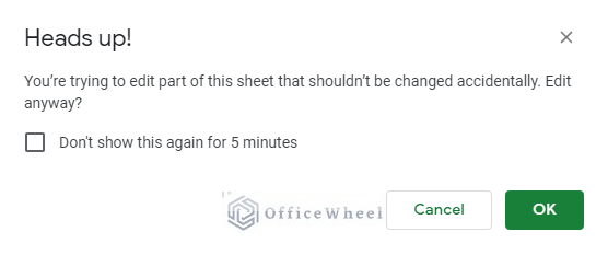
If anyone (owner of the sheet included) moves to change any protected cells, they will be hit with the following warning:
This concludes the basic way to use Protect Range in Google Sheets. Our next section works with protecting an entire worksheet.
Read More: How to Protect Formulas in Google Sheets (2 Quick Ways)
2. Protect an Entire Worksheet in Google Sheets
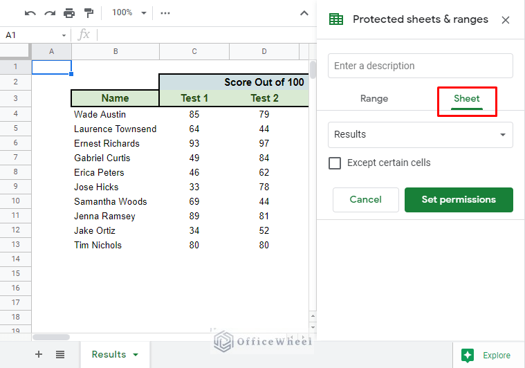
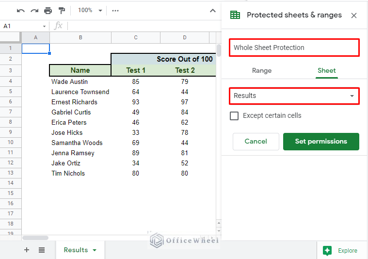
Remember the Sheet option in the Protected sheets & ranges menu? We are going to be using it now.
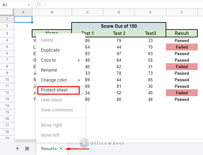
Another way we can directly bring up the Protect Range for whole worksheets in Google Sheets is by using the Sheet tab at the bottom of the page, called Protect sheet.
Back in the Protected sheets & ranges window, we have similar sections: the name (optional) and now the sheet name.
You will also notice the Except certain cells checkbox here. Clicking on it will allow you to choose ranges of cells that you want to keep unlocked.
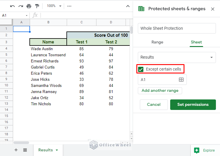
Once you are satisfied with your choices, click Set permissions to move to the next stage.
The Range editing permissions are the same as we have discussed in the previous section. You can go have a look at it in detail.
Read More: Protect Sheet From View in a Google Spreadsheet (2 Ways)
Final Words
As we have seen, it is quite easy to implement Protect Range in Google Sheets, both for your cells or entire worksheets. We hope the guide we have presented comes in handy for you to understand it. For a more in-depth guide, please visit our How to Lock Cells in Google Sheets article.
Please feel free to leave any queries or advice you might have for us in the comments section below.