The Custom Number Format feature of Google Sheets serves to add additional formatting rules to number values in the application.
These formatting rules are simply an additional visual layer that is used to transform a numerical value to be presentable in ways required by the user. This formatting does not change the number values.
In this article, we will dive deep into this feature and break it down to understand it better so that you can start creating your own custom number formats.
The Basics of Custom Number Format in Google Sheets
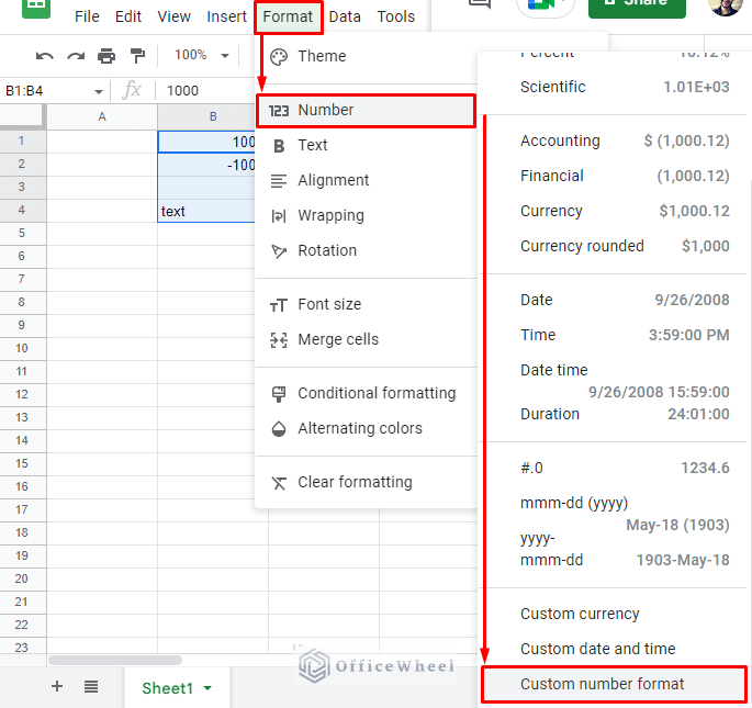
We can navigate to the Custom number format option in Google Sheets from the Format tab:
Format > Number > Custom number format
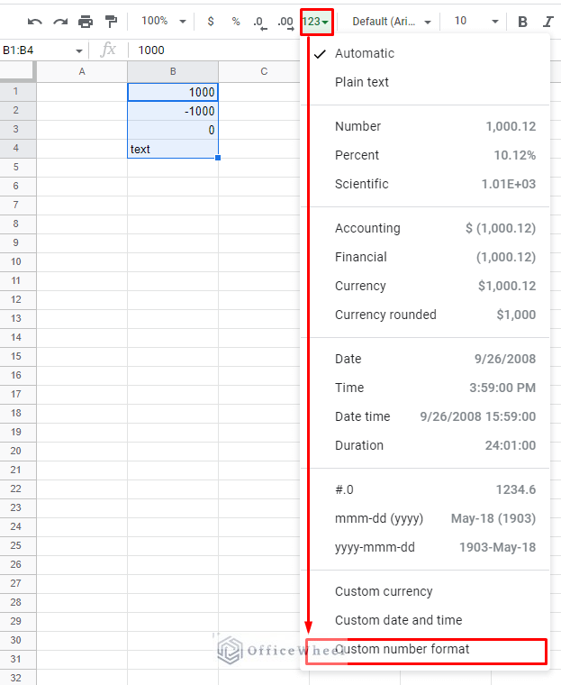
Alternatively, you can also reach this option from the More formats menu in the toolbar:
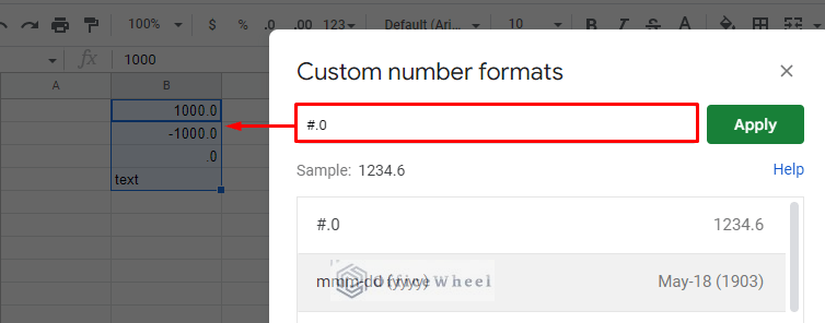
This will open the Custom number formats window:
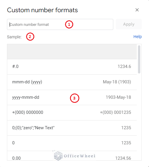
- The field where you enter the number formatting formula.
- The Sample section shows what the outcome of the formula will look like.
- Here you’ll find existing custom formats for number values.
The Structure of Custom Number Format in Google Sheets
The custom number format can be split into 4 data types:
- Positive
- Negative
- Zero
- Text
Each of these data types can be formatted individually and is separated with semicolons (;) in the formula field. Semicolons are also used to separate different conditions in custom number formatting, we will see their use later in this article.
In a general scenario, users usually input a simple number format. These are taken as default and applied to both positive and negative numbers.
For example, applying the “#.0” format to the selected cells gives us all number values with 1 decimal place. Click Apply once the format formula is entered:
On the other hand, we can customize each data type individually using a custom number format. For example, let’s apply the following condition:
#.0;(0);"-";"Not a Number"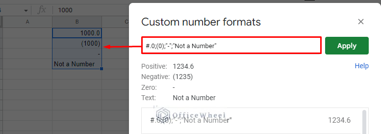
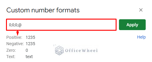
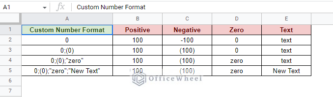
Do you have to use all 4 customization fields?
No. It is not necessary to use all 4 fields when applying a custom number format in Google Sheets.
Generally, when a user inputs a number format, the first three fields are included by default since the fourth field only works with text values.
However, to customize later fields, a user must occupy the previous fields first.
Here’s a simple table showing the results of adding the rules one by one:
Common Custom Number Format Rules in Google Sheets
There are many rules (application of special symbols) that can be used to format numbers, but the following are the most commonly used. And for most cases, these are enough.
The Hash/Pound (#) Rule
The hash symbol (#) rule is used when we want to define a number value as optional. This means that the number presence is optional and insignificant zero (0) values will not be counted.
Here’s what happens when we set the custom number format to only #:
The Zero (0) Rule
The zero (0) rule is the fundamental number rule where all numerical values are counted, even insignificant zeroes.
Here’s what happens when we only input 0 in the custom number format field:
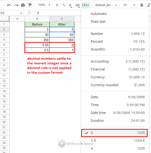
A point to note here is that the decimal numbers are counted to their nearest integers. This is because a rule for decimal numbers was not included in the custom number format.
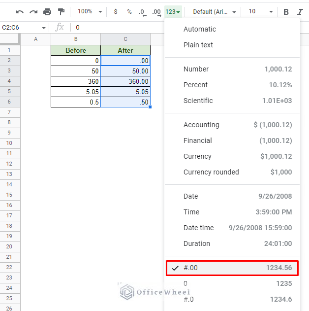
To include decimal points, we must include a period (.) before the number of decimal points represented by 0.
For example, the custom formula to convert numbers to 2 decimal places can be:
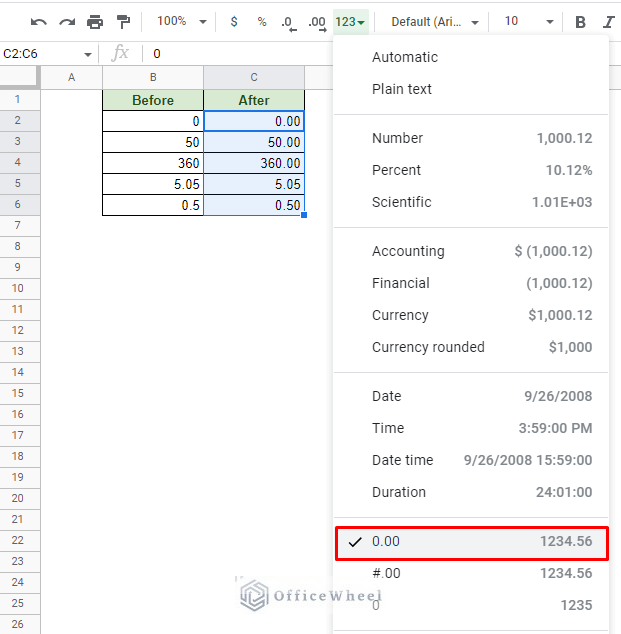
#.00This does not count any insignificant 0 values.
0.00This counts the insignificant 0 values.
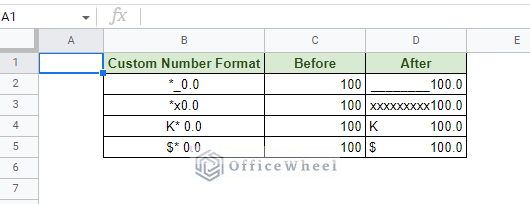
The Asterisk (*) Rule
The asterisk (*) symbol is used to define a repetition in custom number formats.
Any character that is input after an asterisk is repeated the entire width of the cell or until a number format. This also includes whitespaces.
The following image shows some results of using the different asterisk rule formats on the same number:
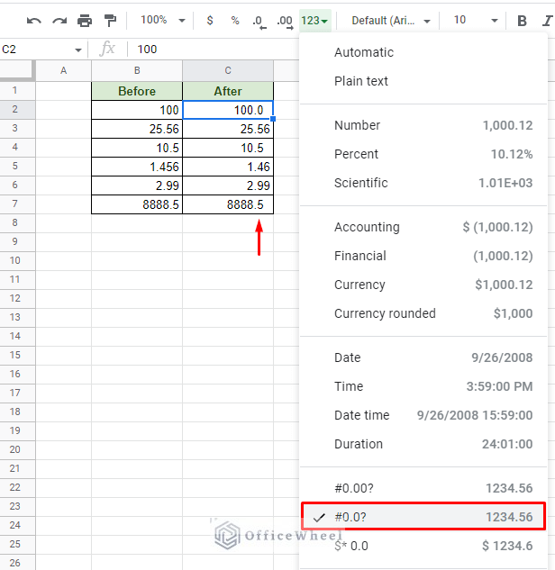
The Question Mark (?)
The question mark (?) symbol is primarily associated with alignment. But not just any alignment, it’s the decimal place alignment at the end of a number value.
Let’s see what happens when we apply the following custom number format:
#0.0?The results:
4 Examples Using Custom Number Format in Google Sheets
1. Format Negative and Positive Numbers with Different Colors
Let’s start with something simple. Let’s say we have the following dataset and want to format positive and negative numbers in different colors in a column.
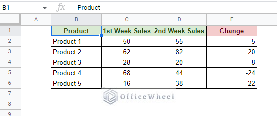
We will apply a custom number format for the values in the Change column.
All we have to do is set the color inside square braces for the Positive and Negative fields of the custom number format. Let’s apply Green for positive numbers and Red for negative ones.
The custom number format formula will be:
[green]0;[red]0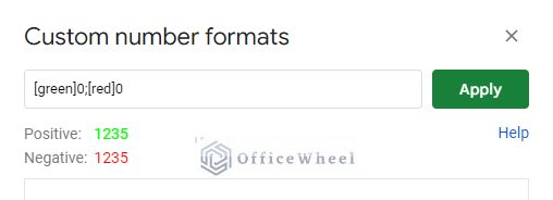
The result:
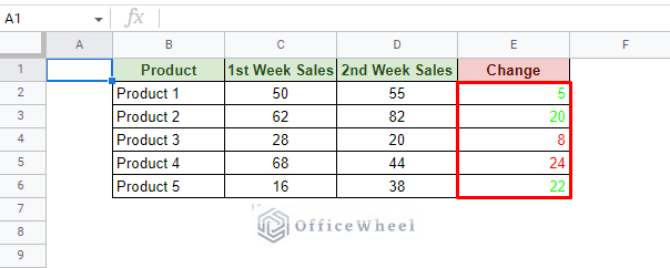
Looks fine, but let’s add a bit more flair to the formatting.
We want to add an increase or decrease symbol next to the results depending on the positive and negative values respectively.
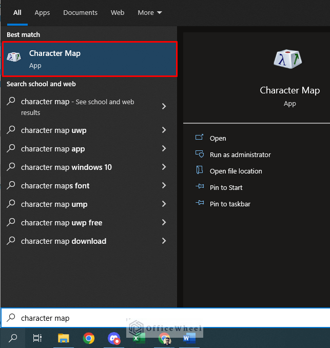
To do that, we must first copy the symbols over from the “Character Map” app in Windows or from the browser.
Step 1: Find the Character Map app in the Windows Search Bar. You can also search for it online.
Step 2: Find and copy the symbols over to the worksheet.
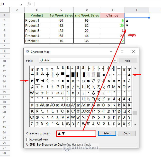
Step 3: Include the symbols in the custom number format formula accordingly. Add a whitespace if necessary.
[green]0" ▲";[red]0" ▼"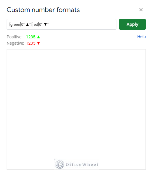
Step 4: Click Apply to see the results.
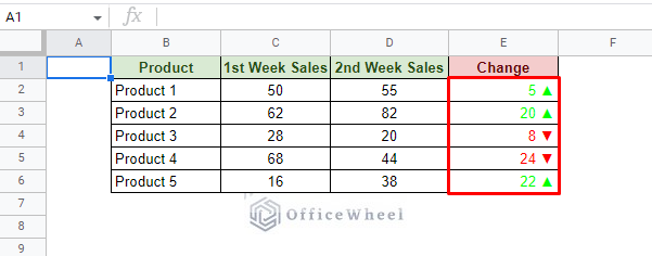
Note: Make sure to move or remove the symbols from the worksheet after you are done.
2. Add Currency Symbol to the Beginning of the Cell
The following is a sample balance sheet going through the expenditures and savings in three months:
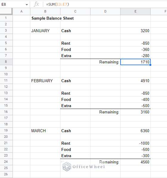
On its own, we cannot value the numbers without the proper currency symbols. We also don’t want the symbols to be adjacent to the numbers but to be at the beginning of the cells.
That said, let’s use the custom number format feature of Google Sheets to format these cells to Euros (€).
We will also implement the asterisk (*) rule to keep the currency symbol and the value separate.
Let’s also go an extra step and remove the negative symbols and leave parentheses instead.
Thus the format formula will be:
€* 0;€* (0)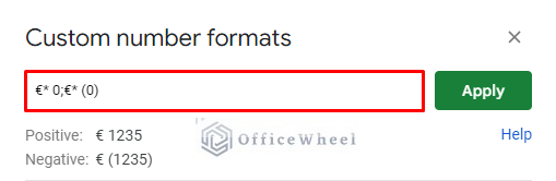
Click on Apply to see the results.
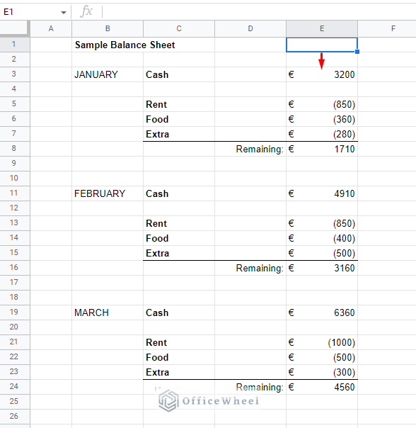
As you can see, the formulas in the cells are not affected and the cells where the format is not applicable are left untouched.
3. Format Dates Using Custom Number Format
Dates in Google Sheets can take on various valid formats. But sometimes, converting one format to another can make it change to a text value as we see with the TEXT function.
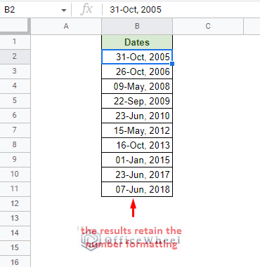
However, the same formatting formula used in TEXT can also be applied as a custom number format. The advantage of this is that the result will remain a number!
Here are a few dates in their standard formats:
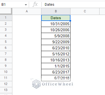
We want to format these dates to Day Number-Partial Month Name, Year. Essentially the dd-mmm, yyyy format. (10/31/2005 to 31-Oct, 2005)
Simply type this formatting in the custom number format field after selecting the date cells:
dd-mmm, yyyy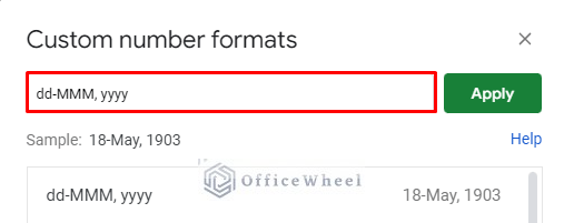
Click Apply to see the result:
4. Format Phone Numbers with Custom Number Format
Phone numbers are another number value that is highly formatted depending on the user and organizational needs.
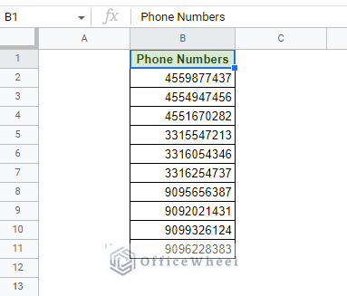
In our sample dataset here, we have some random 11-digit phone numbers that are unformatted:
Phone number formatting is simply about placing the required symbols and numbers in the right positions. A typical phone number is formatted with having its 3-digit region code separate along with symbols like a plus (+) and parentheses.
For example, from 4559877437 to +(455) 9877437
The custom number format formula for this is as simple:
+(000) 0000000Note: Every single digit of the phone number must be accounted for and replaced with 0.
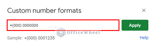
Click on Apply to see the result:
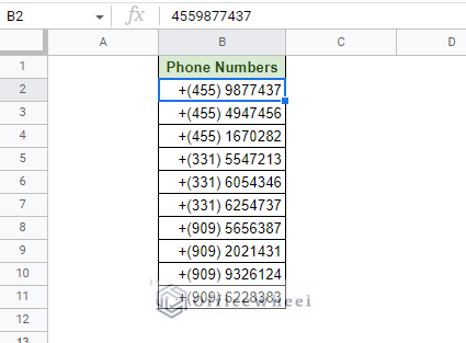
Even with the symbols added, the values are still numbers.
5. Applying Conditional Rules with Custom Number Format in Google Sheets
You can also apply conditional formatting with the custom number format feature of Google Sheets.
Much like regular conditional formatting, the custom number format can take numerical conditions to base the formatting on. Of course, this formatting is only for numerical values.
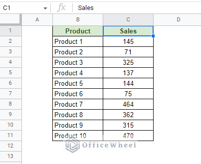
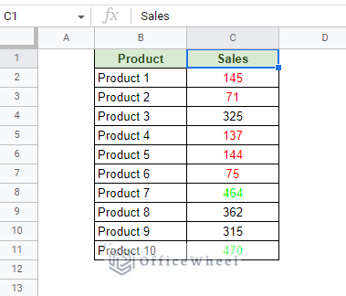
Here, we want to highlight all the Sales values that are above 400 as green and those below 200 as red.
We can enter conditions in the custom number formats field by placing them in square braces. E.g., For values greater than 400, the formula is [>400].
As for applying multiple formatting conditions, simply separate them with semicolons (;).
So, the final custom number format formula will be:
[>400][green]0;[<200][red]0;0Note: You have to account for numbers beyond the ones that fall in the conditions. The final 0 in the formula represents that.
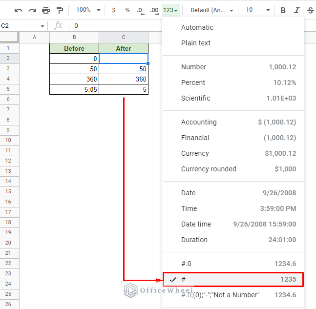
How To Remove Custom Number Format in Google Sheets
Unfortunately, there is no way to remove custom number formats in Google Sheets.
The default option, Clear formatting, does not work with custom number formats.
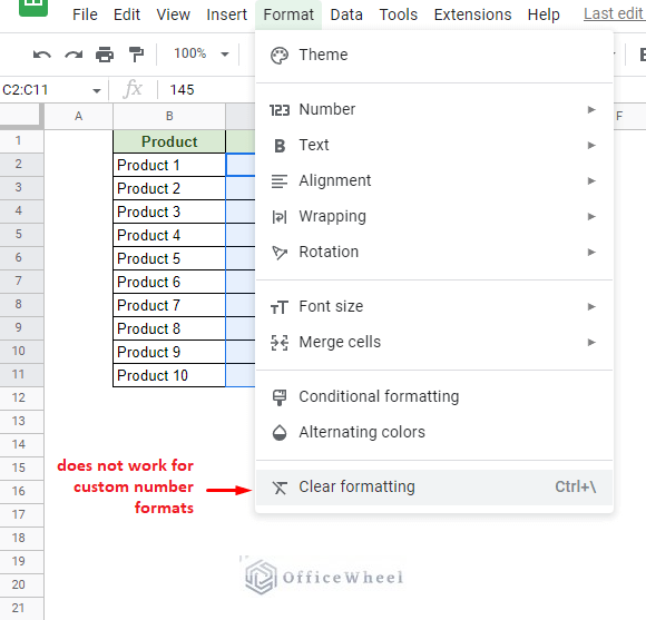
However, we can replace the custom number format with another default format in Google Sheets to remove it.
In the following image you can see that we’ve replaced a custom number format with a default format of Google Sheets:
Final Words
That concludes our simple guide on how to use custom number format in Google Sheets.
It is one of the more versatile formatting features available, and perhaps the most for numbers.
With the help of all the symbolic rules available for the feature, there is virtually no formatting option that this feature is not capable of for numerical values in Google Sheets.
Feel free to leave any queries or advice you might have for us in the comments section below.