The Simple Moving Average (SMA) is a statistical operation that we can use to understand the market trend and in market forecasting. It is very simple to calculate the SMA in Google Sheets. In this article, I will show you how to calculate the simple moving average in Google Sheets.
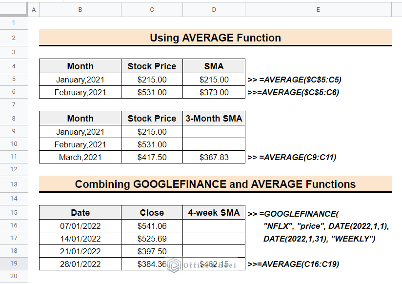
The above screenshot is an overview of the article representing the use of the AVERAGE function and GOOGLEFINANCE function to calculate the simple moving average for different time periods. You will learn more about how to use the functions to calculate the simple moving average in Google Sheets.
What Is Simple Moving Average
A simple moving average (SMA) is a statistical indicator that calculates the average of a set of data over a specified time period. The SMA is calculated by adding up the data points for a given time period and then dividing that sum by the number of data points in the time period. For example, if you wanted to calculate the SMA for a stock’s closing price over a period of 20 days, you would add up the stock’s closing price for the past 20 days and then divide that sum by 20 to get the SMA. The SMA is a useful tool for identifying trends in data and can be used in various applications, including financial analysis and forecasting.
2 Suitable Methods to Calculate Simple Moving Average (SMA) in Google Sheets
The SMA is a crucial market indicator that is also very simple to calculate. You can use the AVERAGE function to calculate SMA. Additionally, you can review market trends by using actual stock prices or closing prices of numerous internationally renowned companies by using the Google Sheets function GOOGLEFINANCE.
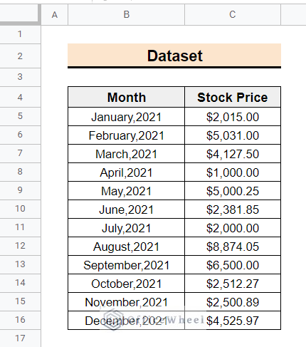
Suppose you have a dataset of the monthly stock price of a company for the year 2021. Now you need to calculate the Simple Moving Average for different specific time periods to realize the market trend and market forecasting.
1. Using AVERAGE Function
You can simply calculate the SMA using the AVERAGE function. Follow the below steps to calculate SMA using the AVERAGE function.
📌Steps:
- To calculate the SMA for every month, first of all, select cell D5 and enter the following formula. This formula determines the SMA for the month of January 2021.
=AVERAGE($C$5:C5)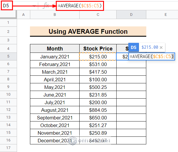
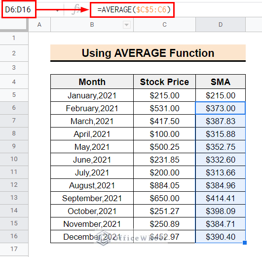
- Then, use the fill-handle tool to copy the formula throughout the column. We can see that the simple moving average has been determined for each month.
- Here, the D6 cell represents the SMA for 2 months. Cell D7 similarly indicates a 3-month SMA, and the cells after it does the same.
- Now to find the SMA for 3 months interval, use the following formula in the E7 This formula will determine the SMA for the first 3 months.
=AVERAGE(C5:C7)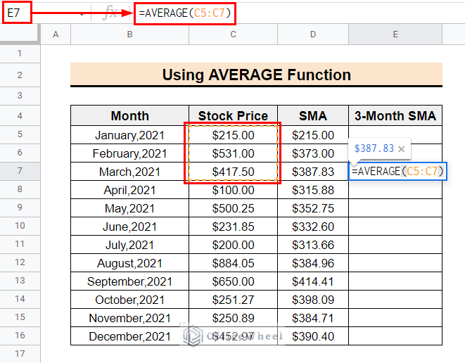
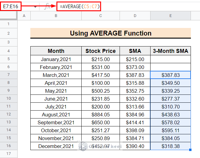
- Afterward, use the fill-handle tool to copy the formula to the following cells. Each cell in the 3-Month SMA column represents the SMA for three months from the current month to the two months prior.
- Here, the first two cells in the 3-Month SMA column in this example are empty because there aren’t enough cells in those regions to calculate the SMA for three months.
Read More: How to Find 200-Day Moving Average in Google Sheets (2 Ways)
2. Combining GOOGLEFINANCE and AVERAGE Functions
You can review the market trend by calculating the SMA of real stock or close prices of different international companies. The Google Sheet function GOOGLEFINANCE allows you to use real stock prices or closing prices for a variety of well-known global corporations so you can review their market trends. This function fetches financial data from the Google Finance website.
Suppose you need to calculate the simple moving average to review the market trend of Netflix Inc. Now to fetch the weekly close price and calculate the SMA follow the below steps using the functions GOOGLEFINANCE and AVERAGE.
📌Steps:
- At the beginning select cell B4 and enter the following formula to fetch the weekly close price of Netflix Inc. The formula will automatically retrieve the weekly close price of Netflix Inc. from January 2022 to April 2022 in a tabular format, as shown in the image below.
=GOOGLEFINANCE("NFLX", "price", DATE(2022,1,1), DATE(2022,4,31), "WEEKLY")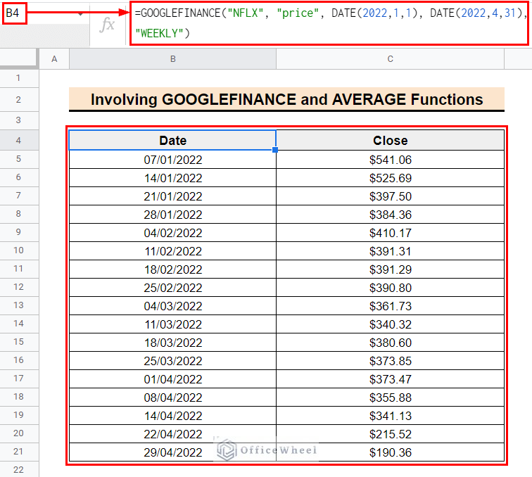
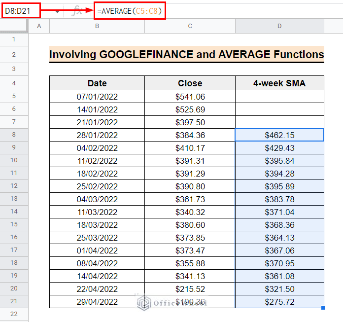
- Now to calculate the SMA for a 4-Week frequency select cell D8 and enter the following formula.
=AVERAGE(C5:C8)
- Then, use the fill-handle tool to copy the fill-handle tool to copy the formula to the following cells. As we can see this formula will produce the 4-Week SMA column representing the SMA for four weeks from the current week to the two weeks prior. The first three cells in the 4-Week SMA column in this example are empty because there aren’t enough cells in those regions to calculate the SMA for four weeks.
- Similarly, we can find the SMA for eight weeks using the following formula in cell E12.
=AVERAGE(C5:C12)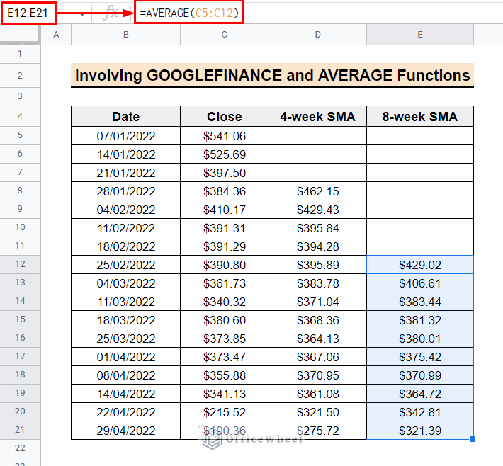
Read More: How to Find 7-Day Moving Average in Google Sheets
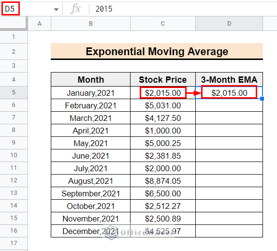
How to Calculate Exponential Moving Average in Google Sheets
The Exponential Moving Average (EMA) is similar to SMA as both are used as indicators of market trends. But there is a slight difference between them. SMA averages prices over the chosen timeframe, whereas EMA gives more weight to recent prices. The EMA calculates the moving average of a range of data. But here a weight factor is added to each data point so that the weights decrease exponentially as the data points move further away from the current value. Formula to calculate the EMA,
Here, where datacurrent is the current data value; EMAcurrent and EMAprevious are the current and the previous exponential moving averages respectively and k is the desired number of periods.
Follow the below steps to calculate the EMA.
📌Steps:
- In the beginning, enter the EMA value in cell D5 to be equal to the value in cell C5 because the EMA of 1st entry remains the same as the price.
- Then, use the following formula in cell D6 to calculate the EMA for 3 months.
=D5+((2/4)*(C6-D5))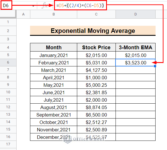
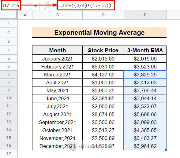
- Afterward, using the fill-handle tool copy the formula to the following cells.
- In a similar procedure, you can calculate the EMA for 5 months using the following formula.
=(C6-E5)*(2/6)+E5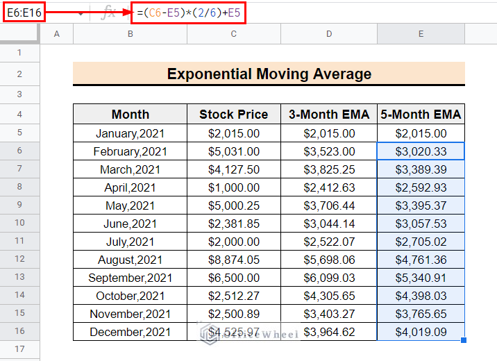
Read More: How to Find 50 Day Moving Average in Google Sheets
Things to Remember
- Choose the data range based on the time interval needed to calculate the simple moving average.
- While using the GOOGLEFINANCE function you can get data for time intervals DAILY and WEEKLY.
Conclusion
Following the methods hopefully, now you can calculate the simple moving average in Google Sheets. If you have any query or suggestion please write it in the comment section. For more useful articles related to Google Sheets please visit the Officewheel site.