Google Sheets is becoming more and more popular day by day as a leading spreadsheet application. It is mainly due to the availability of a wide range of functions including some very useful exclusive functions. The LEFT function in Google Sheets is one of those functions. It can be applied to serve various purposes. In this article, we will try to demonstrate the anatomy of this function. We will also illustrate some practical examples to use this function. Hopefully, this will help you to learn about this function in detail.
A Sample of Practice Spreadsheet
What Is LEFT Function in Google Sheets?
The LEFT function returns a specific number of characters or substrings from the beginning of values or strings.
Syntax
The Syntax of the LEFT function is as follows.
LEFT(string, [number_of_characters])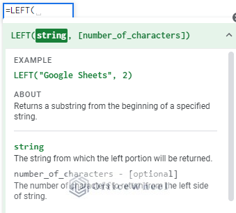
Arguments
| ARGUMENT | REQUIREMENT | FUNCTION |
|---|---|---|
| string | Required | The reference string i.e. texts, numbers, or other values; a portion from the left or beginning of this will be returned. |
| number_of_characters | Optional | This is the specific number of characters that the function will return from the beginning of the string. The default value is 1. Entering 0 will return an empty string. |
Output
The formula LEFT(“ABCDEFGH”, 3) will return ABC as the first 3 characters from the left of ABCDEFGH is ABC.
5 Suitable Examples of Using LEFT Function in Google Sheets
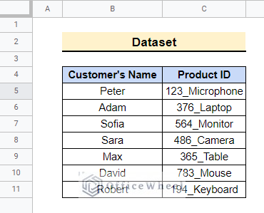
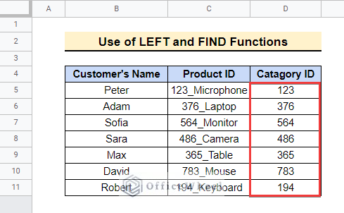
Let’s have a look at the simple dataset below. In the dataset, we have some Customer Names and Product IDs. We will use the Product IDs as the String argument of the LEFT function to demonstrate some practical applications of the function.
1. Get Characters from the Beginning of Strings
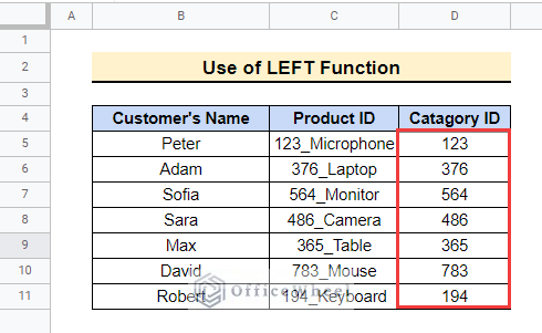
Notice that the Product IDs contain 3-digit numbers which are the Category IDs of the corresponding products. Here, we will show how to use the LEFT function to get those Category IDs from the beginning of the strings. Follow the steps mentioned below for that.
📌 Steps:
- First, select cell D5 in the Category ID Then enter the formula given below.
=LEFT(C5,3) 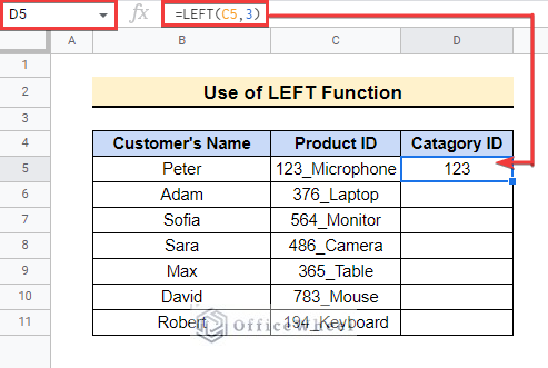
- Here the LEFT function returns 3 characters from the beginning of the string in cell C5.
- Now you need to drag down the Fill handle icon to copy the same formula into the other cells.
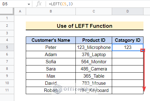
- In the end, you will get the Category IDs from all of the Product IDs as follows.
Read More: How to Use Formula to Highlight Duplicates in Google Sheets
2. Return Substrings from Multiple Texts
Here, we will show how to use the LEFT function along with the ARRAYFORMULA function to return substrings from multiple strings at once. The ARRAYFORMULA function converts a simple formula to an arrayformula. This enables the formula to return multiple results at once. This way you won’t need to drag the Fill Handle icon.
- Apply the following formula to cell D5 to get the same output as before without copying the formula below.
=ARRAYFORMULA(LEFT(C5:C11,3)) 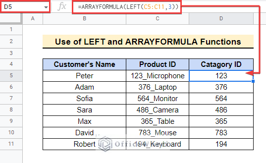
Read More: How to Use ARRAYFORMULA in Google Sheets (6 Examples)
3. Find and Extract Characters from Strings
Now we will combine the LEFT function with the FIND function to find the “_” character in Product IDs and extract the characters before that. Here the case-sensitive Find function finds the position of a character within a string.
📌 Steps:
- First, enter the following formula in cell D5 as shown below.
=LEFT(C5,FIND("_",C5)-1)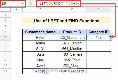
- The position of the “_” character in 123_Microphone is 4. So FIND(“_”,C5)-1 returns 4 – 1 = 3. Then the final formula becomes LEFT(C5,3) as earlier.
- Now drag down the fill handle to copy the same formula into the cells below.
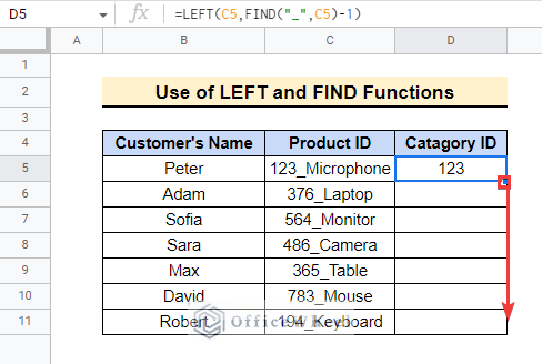
- In the end, you will get the same output as earlier.
Read More: How to Use the Find Function in Google Sheets (An Easy Guide)
4. Search and Return Characters from Texts
The limitation of the FIND function used earlier is that it is case-sensitive. So it can only find exact matches. Suppose you need to find the position of a character whether it is uppercase or lowercase. Then you should instead use the case-insensitive SEARCH function. So here we will use the LEFT function with the SEARCH function to return substrings before the position of the searched character. The steps are as follows.
📌 Steps:
- First, enter the following formula in cell D5 as shown in the following picture.
=LEFT(C5,SEARCH("_",C5)-1)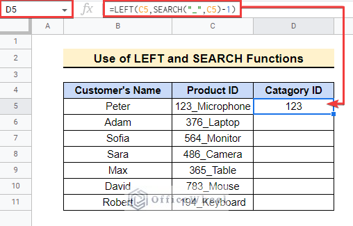
- Here the SEARCH function searches for the “_” character in cell C5 and returns 4 as the FIND function. If you searched for “m”, the function would have returned 5 which is the position of M within 123_Microphone.
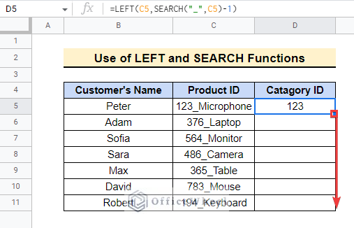
- Now drag the fill handle down to copy the formula to the cells below.
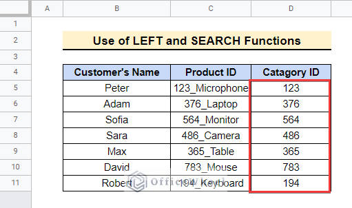
- In the end, the output will be as below.
Read More: How to Compare Text in Google Sheets (3 Easy Ways)
Similar Readings
- How to Create Dependent Drop Down List in Google Sheets
- Format Date with Formula in Google Sheets (3 Easy Ways)
- How to VLOOKUP with Multiple Criteria in Google Sheets
- Remove Everything after Character Using Google Sheets Formula
5. Remove Specific Number of Characters
Finally, we will show how you can use the LEFT function with the LEN function to remove the last 4 characters from the Product IDs. Here the LEN function returns the length of a string i.e the total number of characters within a string. You can implement this method to your own dataset as required.
📌 Steps:
- First, enter the following formula in cell D5 as shown below.
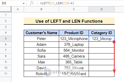
=LEFT(C5,LEN(C5)-4)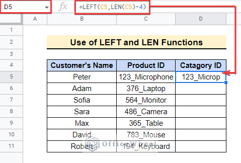
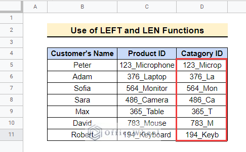
- After that, drag down the Fill handle to copy the formula below.
- As a result, you will get the following output.
Formula Breakdown
➣ LEN(C5)-4: Here the LEN function returns the length of the string in cell C5. So the output of LEN(C5) = LEN(“123_Microphone”) = 13. So the output from LEN(C5)-4 is 13 – 4 = 9.
➣ LEFT(C5,9): Now the LEFT function returns 9 characters from the beginning of the Product ID in cell C5e. 123_Microphone. So the final output is 123_Microp.
Read More: How to Remove Characters from a String in Google Sheets (6 Easy Examples)
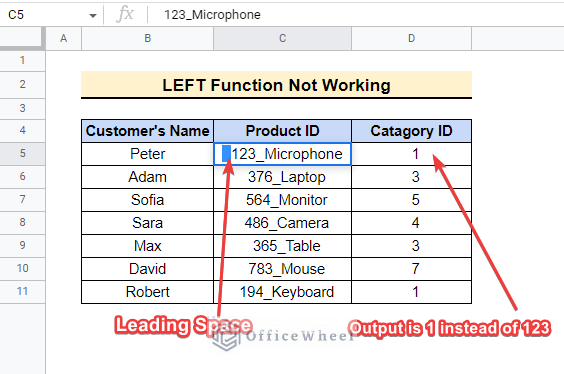
What to Do When LEFT Function Is Not Working in Google Sheets
The examples demonstrated above suggest that we can use the LEFT function for various purposes. But sometimes it may return erroneous results. If there are leading spaces or other invisible characters at the beginning of the string, then the function will return the invisible characters first. So it may seem that the function is returning erroneous results.
- For example, let’s have a look at the following formula. Here the LEFT function is returning 1 instead of 123.
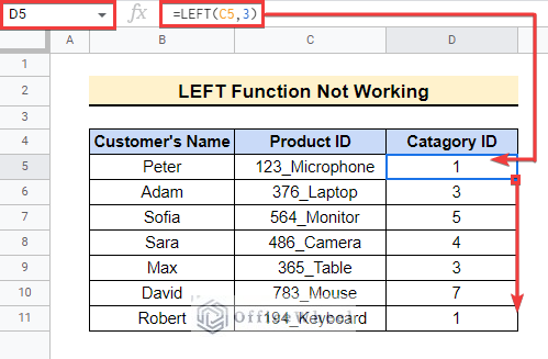
- This is because the Product IDs contain 2 leading spaces. If you double-click on cell C5 and move the cursor at the beginning of the string, you will find the leading spaces. So we are only seeing the last visible character.
- If you remove the leading spaces, then the LEFT function will return the desired results as earlier.
Read More: Remove Everything after Character in Google Sheets
Things to Remember
- Always make sure that your dataset does not have leading spaces if you need to use the LEFT function. Otherwise, you may not get the desired results.
- The LEFT function only returns characters from the beginning of strings.
Conclusion
In this article, we explained the anatomy of and how to use the LEFT function in Google Sheets with various practical examples. Hopefully, the methods will help you to apply the function to your own dataset. Please let us know in the comment section if you have any further queries or suggestions. You may also visit our OfficeWheel blog to explore more Google Sheets-related articles.