In Google Sheets, if you want to calculate a series of averages for a dataset in a fixed period, you can use the Moving Average method. The moving average is basically used in time series data analysis. In this article, we will explore the particular exponential moving average in Google Sheets.
A Sample of Practice Spreadsheet
You can download spreadsheets from here and practice.
What Is Exponential Moving (Rolling/Running) Average?
The Exponential Moving Average or EMA is one kind of moving average that gives more emphasis on recent observations. By using this method you can easily cope with recent trends.
The syntax for Exponential Moving Average is:
- Here, EMACurrent is the current exponential moving average and EMAPrevious is the previous exponential moving average.
- n is the number of periods and XCurrent is the current data value.
Let’s see its application with a simple example:
Step by Step Procedure to Find Exponential Moving Average (EMA) in Google Sheets
To find the exponential moving average in Google Sheets you have to follow three simple steps. First, you have to create a dataset, then apply the EMA calculation formula and finally get the output for the entire dataset.
Step 1: Setting Up Data
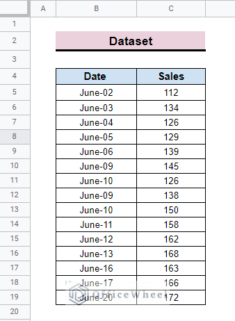
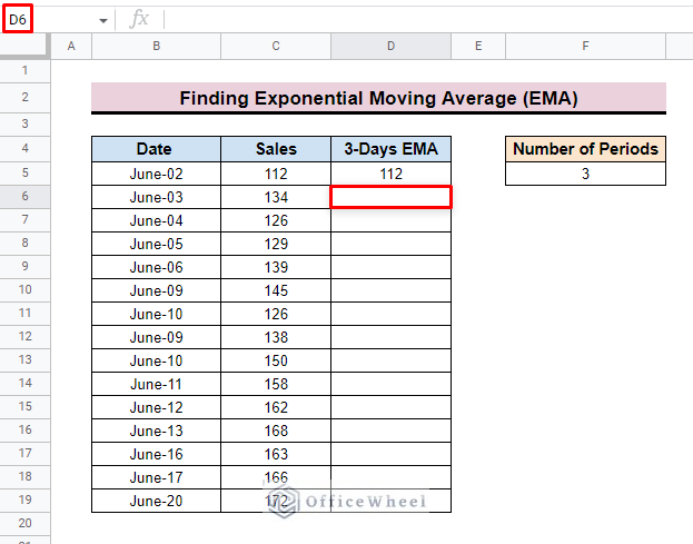
To calculate the exponential moving average first, we develop a dataset.
- The dataset represents the date and sales for June.
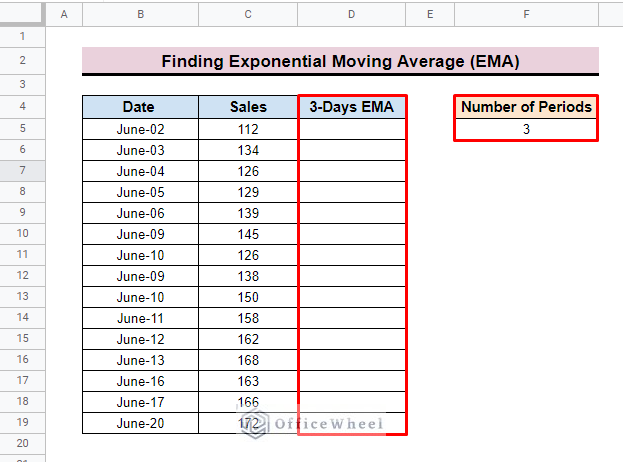
- To apply the moving formula in this dataset we create a new column name 3-Days EMA. As we want to calculate the EMA of 3 days that’s why we also add several Periods cells to specify the period. We add 3 in this cell.
Step 2: Applying the EMA Calculation Formula
To calculate the EMA for the entire dataset now we have to insert the EMA calculation formula,
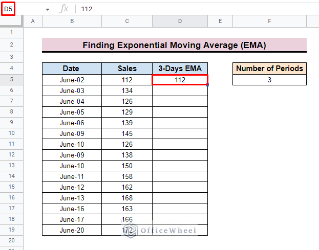
- First, for calculating the 3-day EMA inserts the first value of the dataset as the initial 3-day EMA value. Here, we input 112 in cell D5 as the initial 3-Days EMA value.
- The initial value is not affected by the calculation.
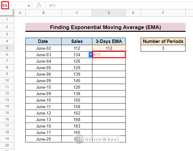
- Now select cell D6 to apply the calculation formula.
- Now, insert the D5 cell as the first value of the formula. Here, D5 represents the previous EMA value.
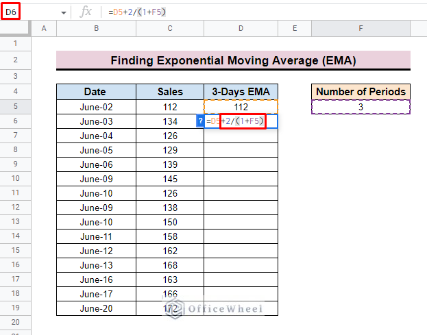
- Then input + symbol and after that 2/(1+F5) where F5 is the number of periods.
- This section of the formula is also known as the smoothing constant.
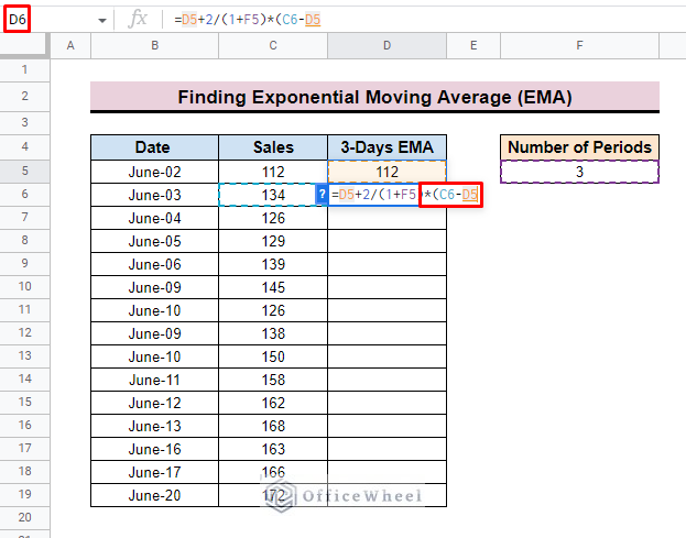
- After that insert the multiply sign (*) and also subtract between C6 and D5.
- Here, C6 is the current (date) Sales value for the dataset and D5 is the previous EMA value.
Read More: How to Calculate Moving Average in Google Sheets (2 Ways)
Step 3: Finalizing Output for Entire Dataset
After applying the whole formula,
- Finally, press ENTER and you will find the EMA value in the selected cell.
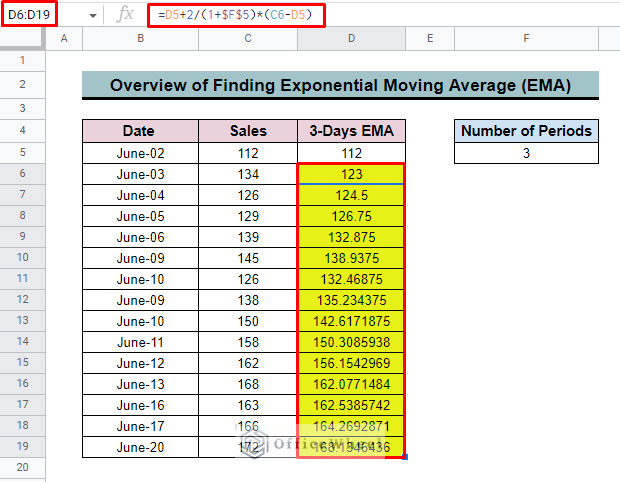
=D5+2/(1+F5)*(C6-D5)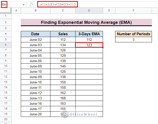
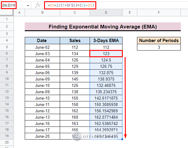
- But before we apply this formula to the rest of the column, we have to make a couple of changes.
- Here, to make the number of period cells constant we add $ before the cell number. So in the formula, it presents like $F$5. So make sure to update.
=D5+2/(1+$F$5)*(C6-D5)- Finally, use the fill handle to apply this EMA formula to the rest of the column.
Find 50-Days Exponential Moving Average in Google Sheets for Registered Company
To calculate the 50-day exponential moving average for any registered company, you can use the GOOGLEFINANCE function in Google Sheets. With the help of this function, you can easily generate a customized dataset by using different parameters in the function.
Step 1: Generating Data with GOOGLEFINANCE Function
The GOOGLEFINANCE function is an applied function in Google Sheets, which presents real-time financial and market data directly in Google Sheets.
The function imports data directly from Google Finance website which is very up-to-date. So, if you want to deal with stock or market finance-related data, this function can be a lifesaver for you.
The general syntax of the GOOGLE FINANCE function is as follows:
=GOOGLEFINANCE(ticker, [attribute], [start_date], [num_days|end_date], [interval])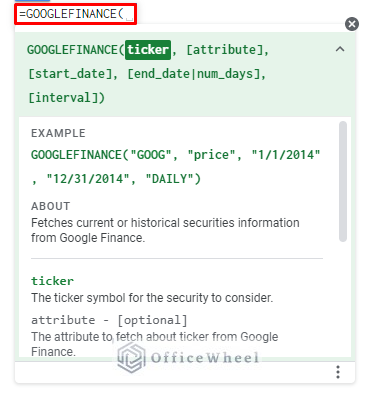
| ARGUMENT | REQUIREMENT | FUNCTION |
|---|---|---|
| ticker | Required | Acronyms to separately identify the designated trade securities. |
| [attribute] | Optional | Types of information you want to display. |
| [start_date] | Optional | To indicate the date from which you want to fetch the data. |
| [num_days|end_date] | Optional | Represents the time frame to extract data. |
| [interval] | Optional | The frequency of picking data. For example, “daily” or “weekly”. |
To get the desired dataset,
- First, we select a ticker which is AAPL, a short form of Apple Inc., then we choose the starting and ending date of the dataset.
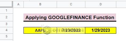
- then select cell B5 and insert the GOOGLEFINANCE function.
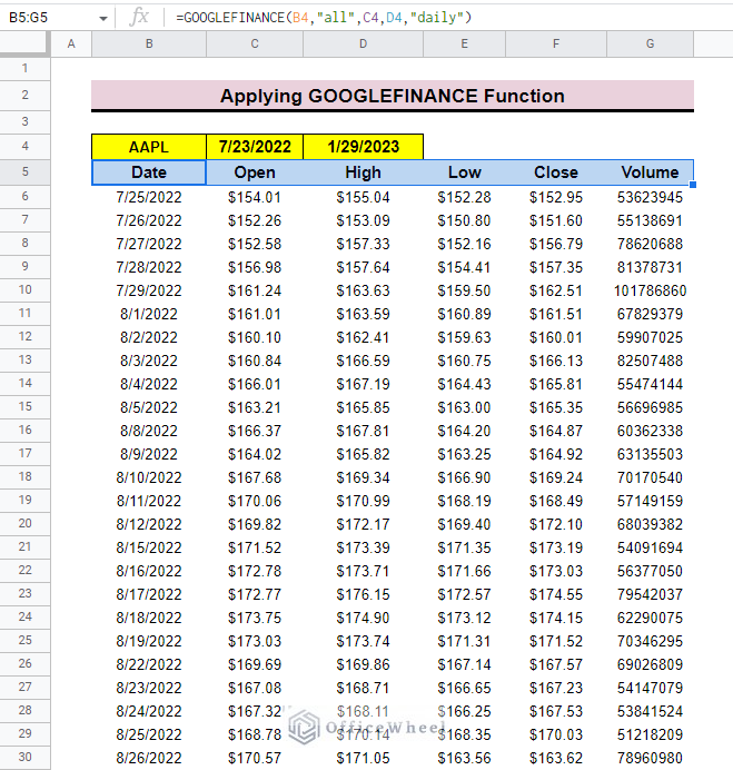
=GOOGLEFINANCE(B4,”all”, C4,D4,”daily”)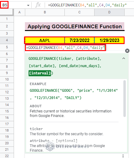
- Finally, press ENTER, and you will find the date-wise dataset.
Step 2: Calculating the First 50-Day Exponential Moving Average
To calculate the EMP for 50 days you have to apply a simple formula.
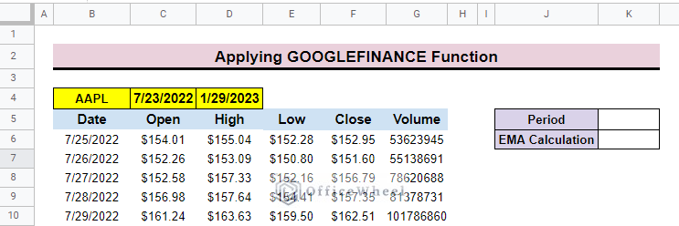
- In the beginning, create two rows presenting the Period and EMA Calculation.
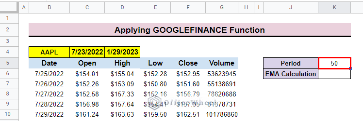
- After that add periods to calculate EMA. Here, we add 50 as we want to calculate 50 days EMA.
- Now add the smoothing constant formula in cell K6.
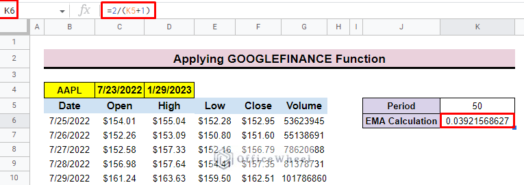
=2/(K5+1)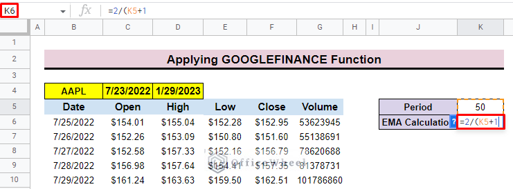
- Then press ENTER to get the calculated smoothing constant value of the EMA.
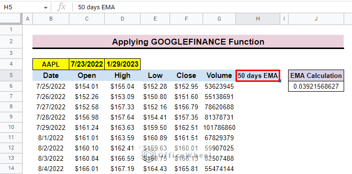
- Now, insert a column named the 50-day EMA that will present the moving average after 50 days.
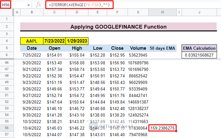
- After that select cell H56 to insert the average formula for the previous 50 days’ close price.
=IFERROR(AVERAGE(F6:F56),””)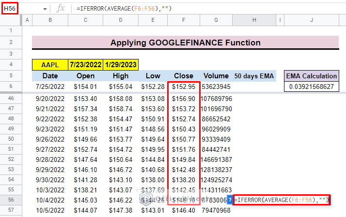
Formula Breakdown:
- F6:F56 represents the range of the value.
- AVERAGE(F6:F56) is the average value of the data range.
- IFERROR(AVERAGE(F6:F56),””) is used to get the accurate result. Returns blank if there is an error.
- In the end, click on ENTER to get the desired result.
Read More: How to Find 50 Day Moving Average in Google Sheets
Step 3: Calculating the Continued 50-Day Exponential Moving Average
After calculating the EMA, now you can calculate the continued 50-day exponential moving average. To do so,
- First, select cell H57 to input the continued exponential moving average formula.
- The general formula for the dataset is:
=((yesterday close price- yesterday EMA)* EMA Calculation)+yesterday EMA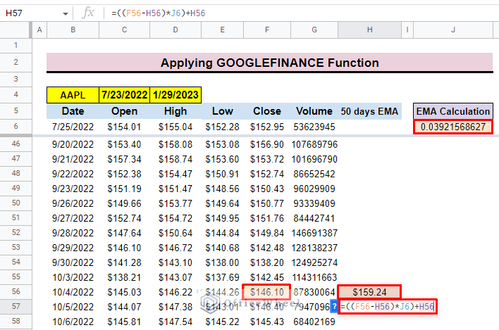
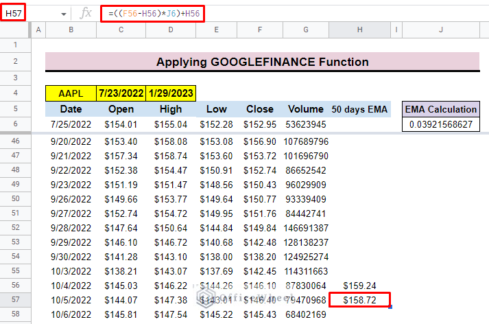
- Finally, press ENTER to get the exponential moving average.
=((F56-H56)*J6)+H56
- Additionally, insert the IFERROR function to get the exact result and avoid errors for the dataset.
=IFERROR((((F56-H56)*J6)+H56),””)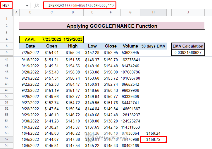
Read More: How to Find 7-Day Moving Average in Google Sheets
Step 4: Finalizing Table
To get the EMA for the entire dataset just drag down the fill handle and you will find the EMA for the entire dataset.
- Here, for the entire column, the EMA Calculation cell is constant. That’s why we use $J$6 in the formula for the entire column. The $ symbol before any cell number will lock the cell in the formula and make the cell absolute.
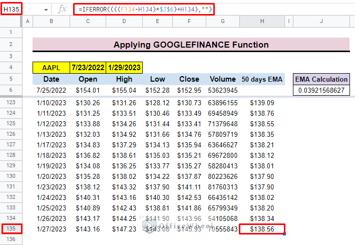
=IFERROR((((F56-H56)*$J$6)+H56),””)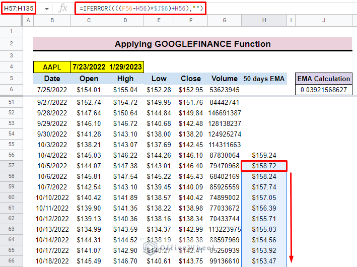
- Additionally, you can find the formula at the end of the dataset.
Things to Remember
- Insert the formula carefully.
- You can apply the second method for any number of days you want.
- For large datasets, always combine the main formula with the IFERROR function to avoid errors.
Conclusion
We believe this article can help you to calculate the exponential moving average in Google Sheets. If you are keen to learn more about different functions in Google Sheets you can visit the OfficeWheel website and enhance your proficiency.