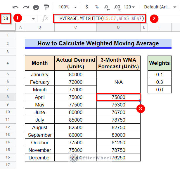
Weighted Moving Average (WMA) is a statistical parameter that we frequently use in business and scientific research. We use it as an indicator of trend direction which we utilize to make critical decisions. In this article, I’ll demonstrate 3 simple ways to calculate the weighted moving average of a suitable dataset in Google Sheets. Here is an overview of the result we require.
A Sample of Practice Spreadsheet
You can copy our practice spreadsheets by clicking on the following link. The spreadsheet contains an overview of the datasheet and an outline of the discussed examples to calculate the weighted moving average in Google Sheets.
What Is Weighted Moving Average?
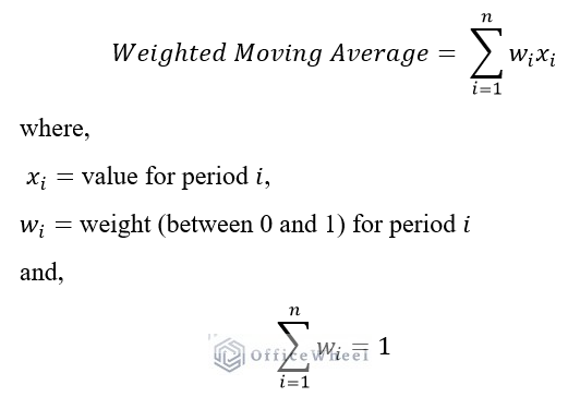
A weighted moving average is a technical indicator that poses more weight on the recent data and less weight on the old data. Few consecutive averages are computed based on a constant size and overlapping successive sets of data to show how the values have moved on average over a certain period of time. The formula to calculate an n-period weighted moving average is following-
3 Effective Ways to Calculate Weighted Moving Average in Google Sheets
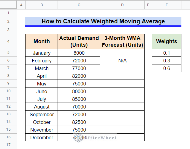
First, let’s get familiar with our dataset. The dataset contains a list of actual demand units for a product for each month of the year. We’ll calculate the 3-month weighted moving average for calculating a demand forecast for each month. The weight of the demands in 3 successive months is 0.6, 0.3, and 0.1 respectively. We will give the largest weight to the most recent data. Since we require the data of 3 months at least to calculate a 3-month moving average, the range D5:D7 is set as N/A. Now, let’s get started.
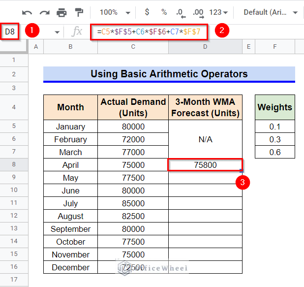
1. Using Basic Arithmetic Operators
First, we’ll manually calculate the moving average for the dataset above using basic arithmetic operators. This method is perhaps the simplest, however, this method is very inefficient if the weighted moving average is calculated for a longer period of time.
Steps:
- Firstly, select Cell D8.
- Afterward, insert the formula below-
=C5*$F$5+C6*$F$6+C7*$F$7- Then, press Enter key to get the required output.
- Now, select Cell D8 again, and then, hover your mouse pointer above the bottom-right corner of the selected cell. At this point, the Fill Handle icon will be visible.
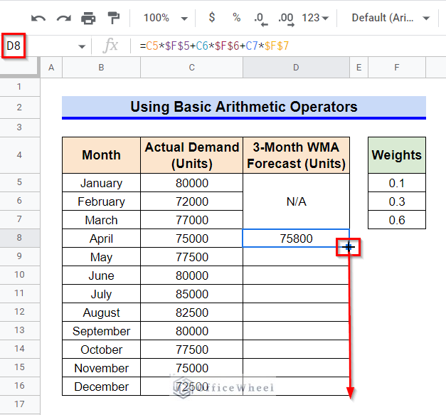
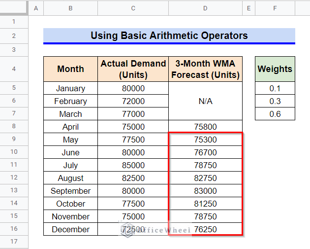
- Use the Fill Handle icon to copy the formula into other cells of Column D.
Read More: How to Find 200-Day Moving Average in Google Sheets (2 Ways)
2. Applying AVERAGE.WEIGHTED Function
Since manually computing with basic arithmetic operators is very tedious for the weighted moving average of a longer period, we can use the AVERAGE.WEIGHTED function instead, which is an exclusive function in Google Sheets. As the name suggests, the AVERAGE.WEIGHTED function is capable of calculating a weighted average for a set of data.
Steps:
- First, activate Cell D8 by double-clicking on it.
- Then, type in the following formula-
=AVERAGE.WEIGHTED(C5:C7,$F$5:$F$7)- Now, get the required output by pressing the Enter key.
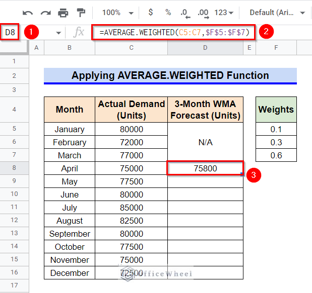
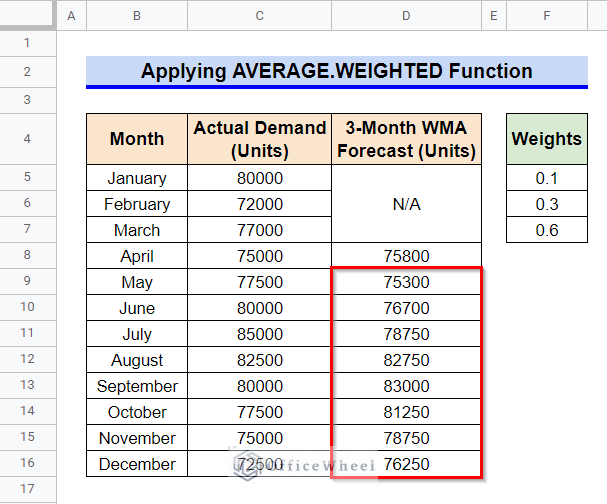
- Finally, use the Fill Handle icon to copy the formula to other cells. And see, it’s giving us the same output as the previous method.
Read More: How to Find 7-Day Moving Average in Google Sheets
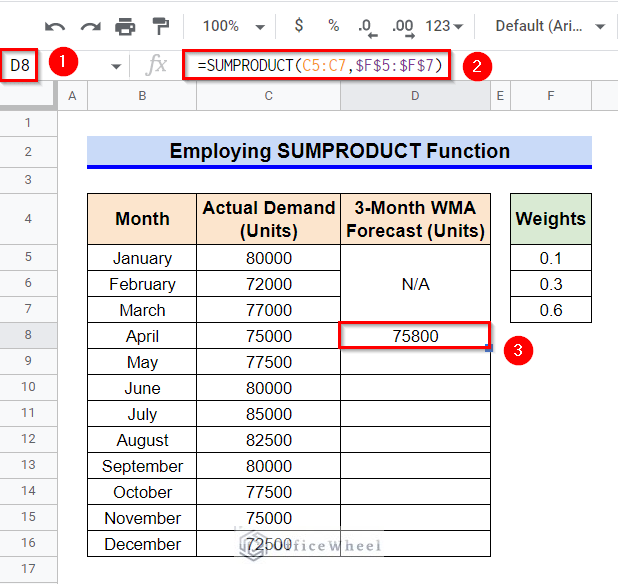
3. Employing SUMPRODUCT Function
We can also use the SUMPRODUCT function to enumerate the weighted moving average of a dataset in Google Sheets. The SUMPORODUCT function is competent in computing the sum of the products of subsequent values in two similar-sized arrays. Now, let’s use it to calculate the weighted moving average for our dataset.
Steps:
- Activate Cell D8 by selecting it first and then using the function key F2.
- Afterward, insert the following formula-
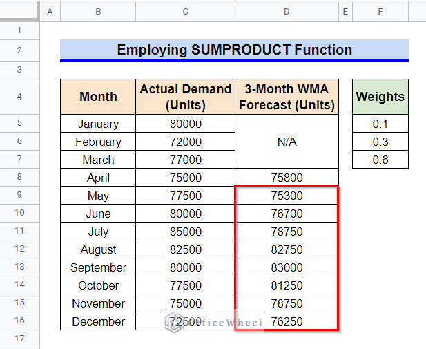
=SUMPRODUCT(C5:C7,$F$5:$F$7)- Consequently, press Enter key to get the required result.
- Finally, copy the formula to other cells of Column D by using the Fill Handle icon.
Read More: How to Find 50 Day Moving Average in Google Sheets
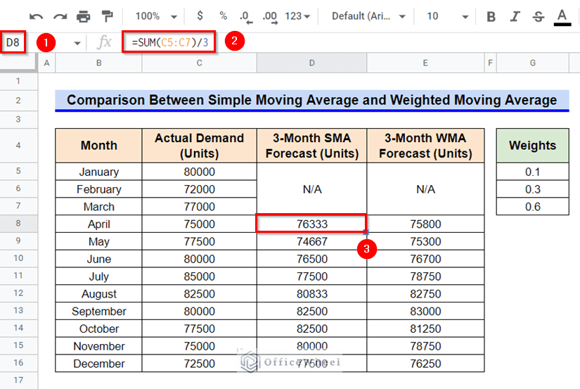
Comparison Between Simple Moving Average and Weighted Moving Average in Google Sheets
Another measure that can depict the moving trend of a dataset is the Simple Moving Average (SMA). The calculation of the simple moving average is very similar to the weighted moving average except, all the values over a time period get an equal weight while computing the simple moving average using the SUM function. Now, a question arises, which tool depicts the moving trend better? Let’s calculate a 3-month simple moving average for our dataset first and then compare it with the weighted moving average. We have added a new column like the following to our dataset for this purpose.

Steps:
- Firstly, select Cell D8.
- Then, type in the following formula-
=SUM(C5:C7)/3- After that, get the required value of SMA by pressing the Enter key.
- Use the Fill Handle icon to copy the formula to other cells.
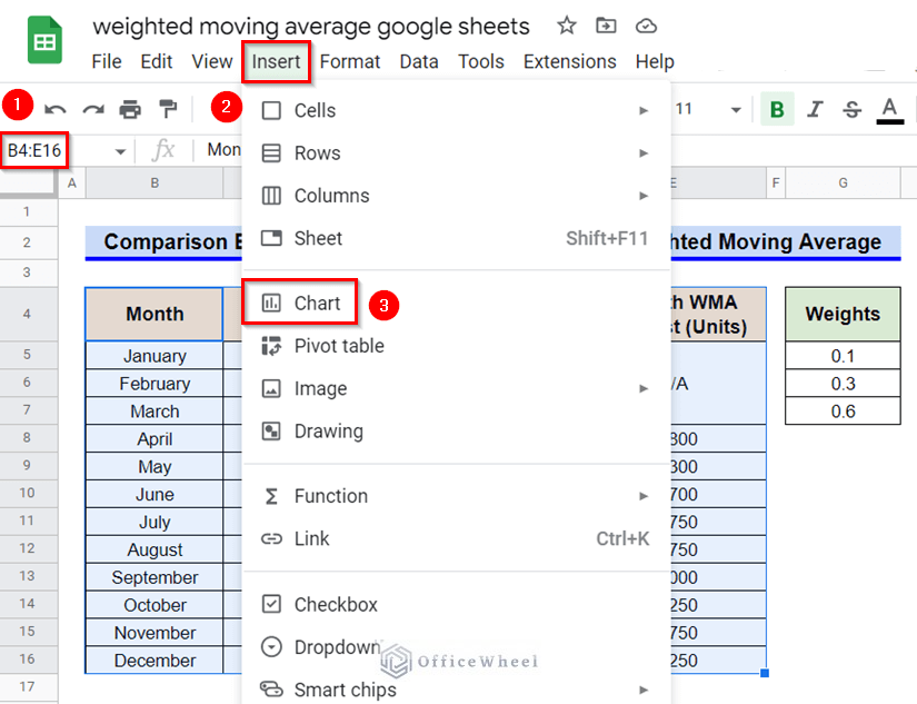
- Afterward, select the range B5:E16 and go to the Insert ribbon.
- Select the Chart command from the appeared options.
- We require a Column Chart for the lucidity of our data. So, whatever type of chart pops up, change it to a Column Chart from the Chart Editor.
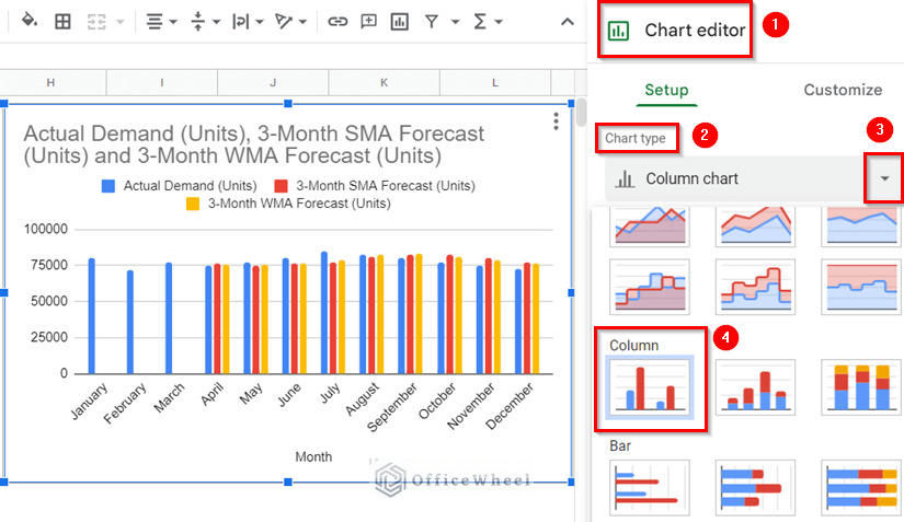
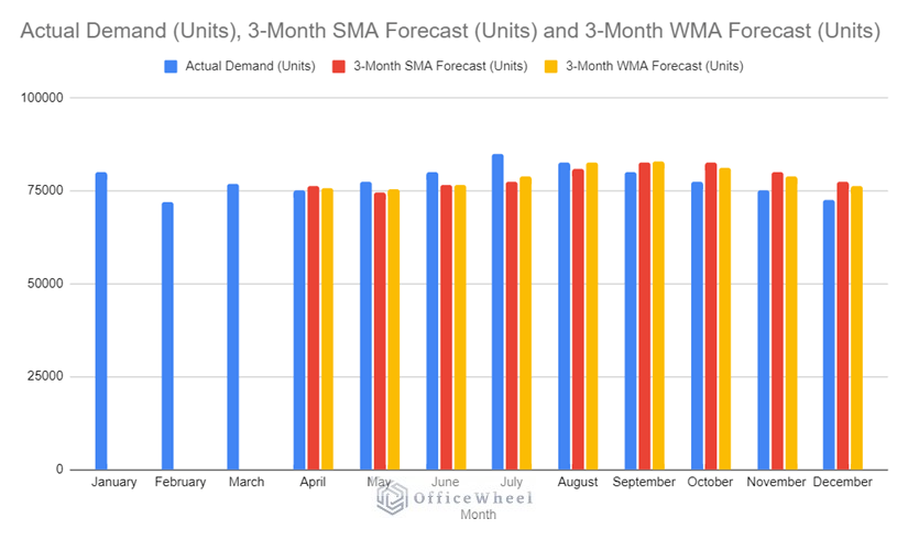
- Now, if you look at the columns, it is clearly visible that the weighted moving average has predicted the trend of actual demand more accurately than the simple moving average.
Things to Be Considered
- The summation of the weights must be equal to 1 while calculating the weighted moving average.
- If the weighted moving average is calculated for a longer period of time, manually computing with basic arithmetic operators is very inefficient and tedious.
- The weighted moving average can depict the trend of a dataset more accurately than the simple moving average.
Conclusion
This concludes our article to learn how to calculate the weighted moving average for a dataset in Google Sheets. I hope the demonstrated methods were ideal for your requirements. Feel free to leave your thoughts on the article in the comment box. Visit our website OfficeWheel.com for more helpful articles.