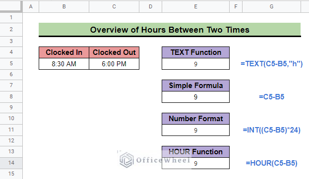
Calculating time duration is very necessary for the business and corporate sections. In Google Sheets, you can easily track your time by applying different formatting and functions to calculate time duration. In this article, you will learn Google Sheets hours between two times in detail.
A Sample of Practice Spreadsheet
You can download the practice spreadsheet from the download button below.
4 Easy Ways to Calculate Hours Between Two Times in Google Sheets
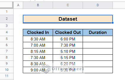
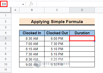
You can apply these techniques to measure time duration in the easiest way. To execute the methods, we develop a dataset that contains Clocked In and Clocked Out times. We have to imply the techniques to find out the Duration.
1. Using TEXT Function
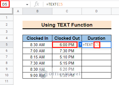
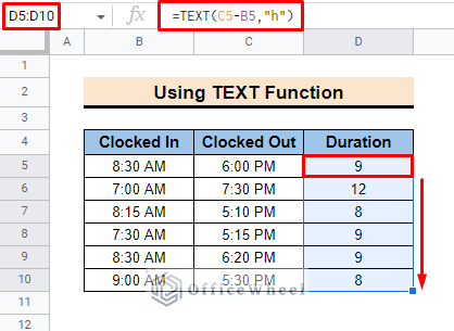
The TEXT function can be applicable for showing time duration in the dataset. To show duration in hours, minutes, and seconds you can use the different TEXT functions. Here, we only show the application of the TEXT function for Hours. To do so,
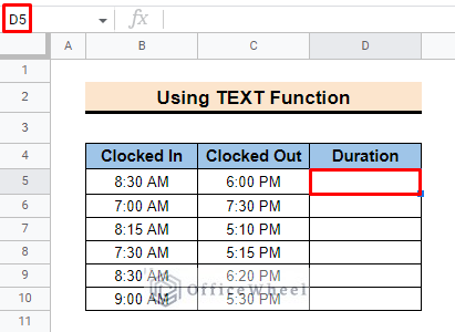
- First select cell D5 to insert the function.
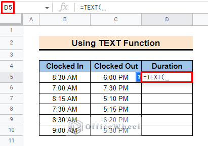
- Then insert the TEXT function in the cell.
- Now, add the Clocked Out time in the function.
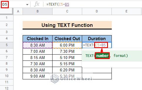
- After that input, the subtraction operator and then the Clocked In time cell.
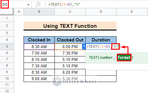
- Then insert “h” for hours as the format of the function.
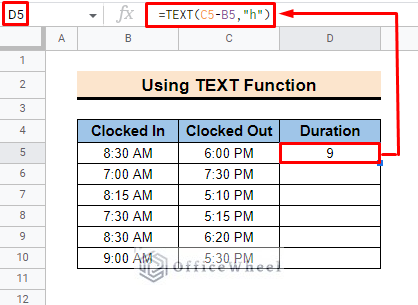
- Finally, press ENTER, and you will find the duration in hours in the selected cell.
=TEXT(C5-B5,"h")- To apply the function to the entire column, use the fill handle and drag it downward.
Read More: How to Calculate Time Between Dates in Google Sheets (6 Ways)
2. Applying Simple Formula
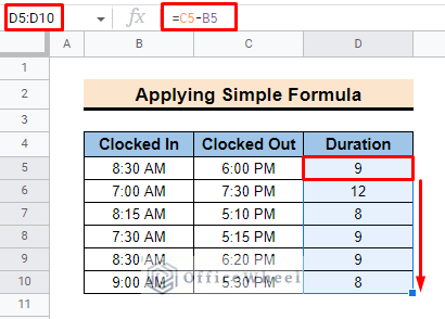
You can simply use the Subtract formula to measure the time duration in the dataset.
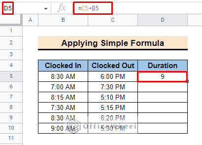
- In the beginning. Select cell D5.
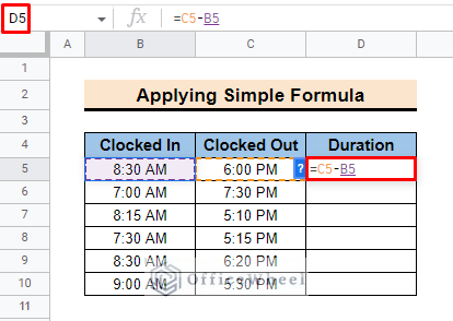
- Then insert the formula to get the Duration.
=C5-B5- Here, C5 is the Clocked Out time and B5 represents the Clocked In time.
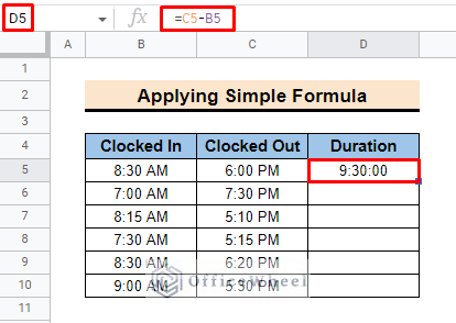
- Now, press ENTER, and you will find the duration of hours with minutes and seconds values.
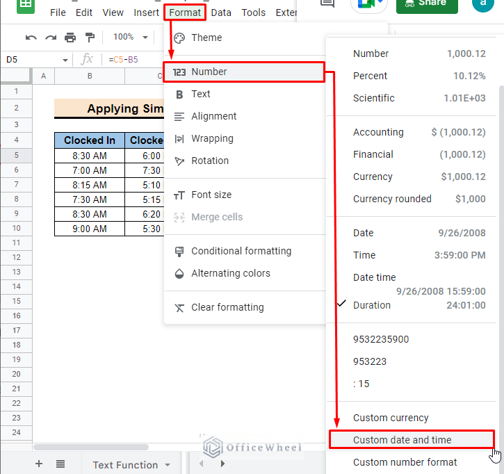
- To get duration only in hours, go to the Format feature and select Number > Custom date and time options.
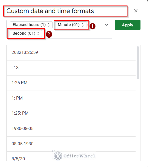
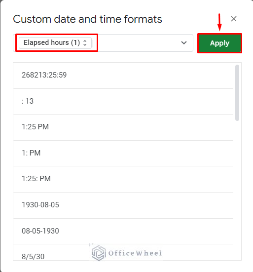
- In the Custom date and time format box, delete the Minute (01) and Second (01) options.
- After that click on Apply.
- Now, you will find only hours in the Duration column.
- In the end, drag down the fill handle to insert the values into the entire column.
Read More: Calculate Number of Years Between Two Dates in Google Sheets
Similar Readings
- Insert Rows Between Other Rows in Google Sheets (4 Easy Ways)
- Difference Between COUNT and COUNTA in Google Sheets
- How to Link Cells Between Tabs in Google Sheets (2 Examples)
- Google Sheets Count Cells Between Two Numbers with COUNTIF Function
- How to Use IF Condition Between Two Numbers in Google Sheets
3. Inserting Number Format
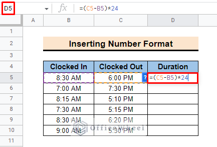
This method works by simply formatting the cells as Numbers,
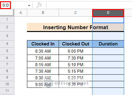
- First, select the cell you want to apply the formatting to. For us, it is the Duration column.
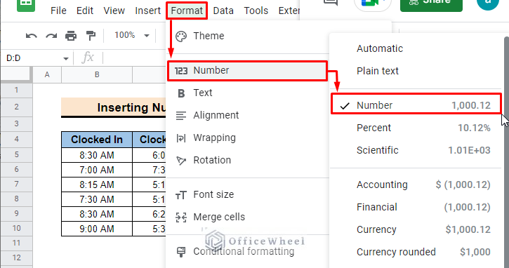
- Then, you have to apply the Number format in the Duration column.
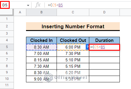
- Then select cell D5 to add the formula.
- Then insert the simple formula.
=C5-B5- Here, C5 is the Clocked Out cell, and B5 is the Clocked In cell.
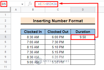
- After that multiply the formula by 24 as we want to get the hour as output.
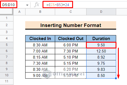
- In the end, click on ENTER and you will find the desired value in the selected cell.
=(C5-B5)*24- Use the Fill handle to apply the formula to the entire column.
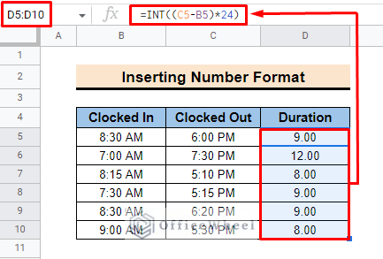
- Additionally, If you want to remove the fraction and only want to show the integers then you can add the INT function with the respective formula.
=INT((C5-B5)*24)Read More: Find Number of Months Between Two Dates in Google Sheets
4. Utilizing HOUR Function
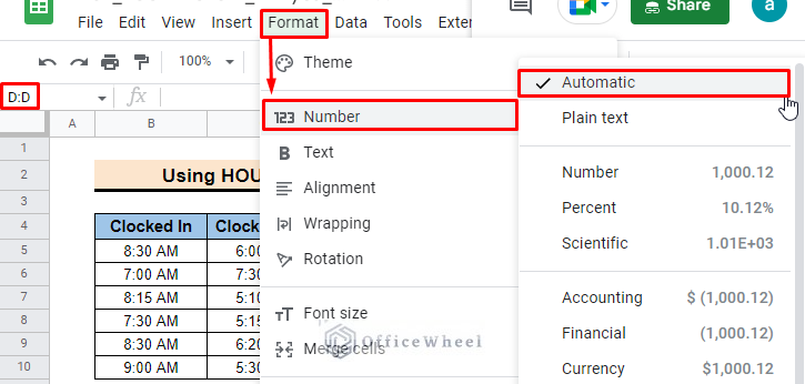
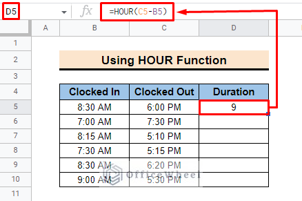
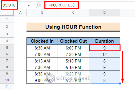
You can apply the HOUR function in the Duration column to get the duration hours. To get the correct result, you have to ensure the Duration column is on number formatting or Automatic Formatting.
To apply the HOUR function,
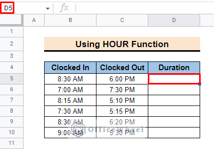
- In the first step, select cell D5.
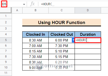
- Then insert the HOUR function in the selected cell.
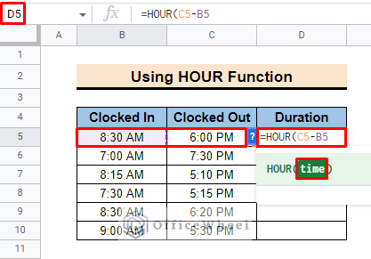
- Now add the cell references as the time argument. Here, we insert the subtraction of C5 and B5 cells as arguments.
=C5-B5- In the end, click on ENTER to insert the function in the selected cell.
=HOUR(C5-B5)- Finally, drag down the fill handle to fill the entire column.
Things to Remember
- You have to care about the formatting of the column to get the exact result.
- Always use the fill handle to apply the formula or function to the entire column.
Conclusion
We believe after completing this article you can develop a clear knowledge of Google Sheets hours between two times. If you are keen to learn more about Google Sheets functions, you can visit the OfficeWheel website and make yourself an expert in Google Sheets.
Related Articles
- How to Find Missing Values Between Two Columns in Google Sheets
- Conditional Formatting Between Two Values in Google Sheets
- How to Find Correlation Between Two Columns in Google Sheets
- Insert Lines Between Cells in Google Sheets
- How to SUMIF Between Two Dates in Google Sheets (3 Ways)
- Calculate Percentage Difference Between Two Numbers in Google Sheets
- How to Filter Between Two Dates in Google Sheets

