Removing duplicates is a common task in Google Sheets or Excel operations. But, the first occurrence of each duplicate generally remains when we use the Remove Duplicates option from the Data ribbon or apply functions like UNIQUE, QUERY, etc. So, when someone wants to remove both (or, all) duplicate rows, previously mentioned methods can not help. However, you can apply the following 2 easy ways to learn how to remove both (or, all) duplicates in Google Sheets.
A Sample of Practice Spreadsheet
You can download a sample of our practice spreadsheet from the following link. The spreadsheet consists of an overview of the datasheet and an outline of the described ways for removing duplicates.
2 Easy Ways to Remove Both Duplicates in Google Sheets
First, let’s get familiar with our datasheet. The datasheet contains the ID, Name, and number of Units sold for several books.
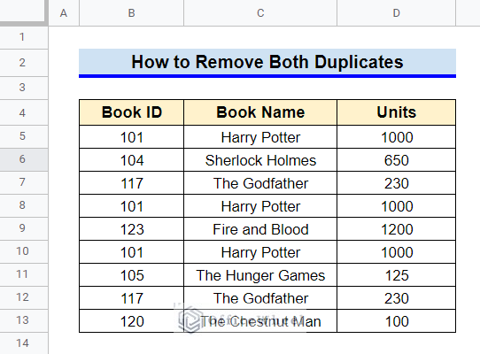
As you can see, several rows are repeated here. Although, we can repeat only cells from a single column in our datasheet. This won’t change our process since we will remove duplicate rows based on one column in Google Sheets. We’ll remove all of these rows. Keep reading to learn how.
1. Using Conditional Formatting and Filter Option
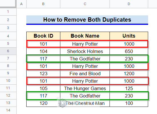
First, we will use Conditional Formatting to highlight the rows that have been duplicated and then use Filter options to remove the duplicates.
Steps:
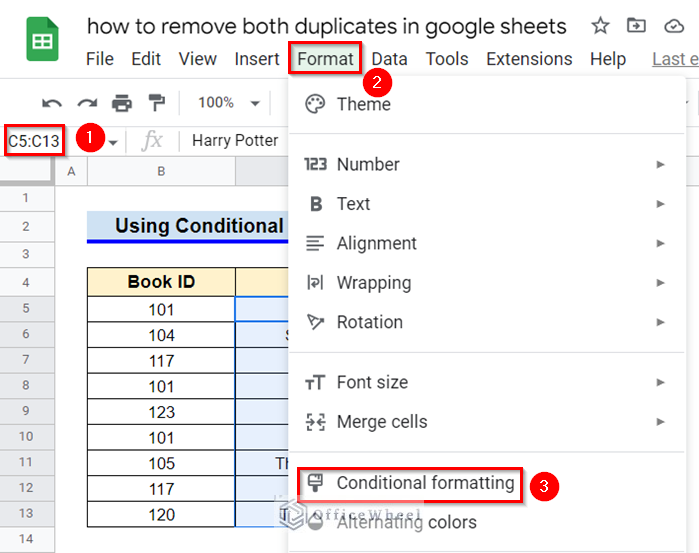
- Select all the cells from any column of the datasheet. I’ll be selecting from Column C. After that, go to the Format ribbon and from there click on Conditional Formatting.
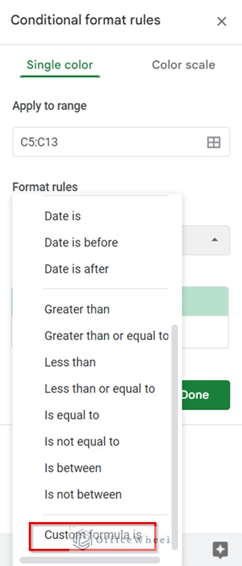
- A sidebar the following will appear. Click on the drop-down icon of Format Rules.
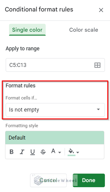
- From the drop-down list, select Custom Formula Is.
- Afterward, type in the following formula in the Values or Formula box and click on Done. Thus we can highlight all the duplicated cells.
=COUNTIF($C$5:C,C5)>1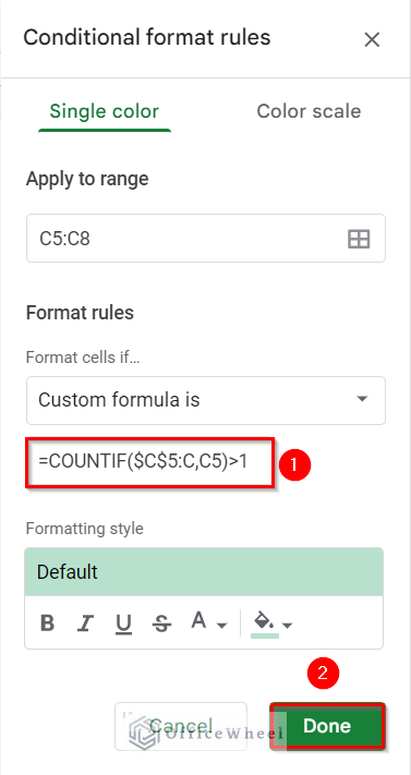
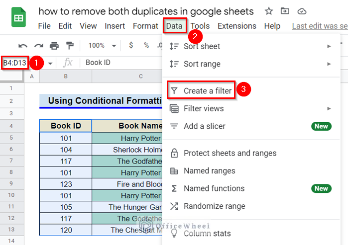
- Now, select the entire data table and then go to the Data From there click on Create a Filter.
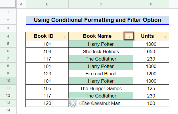
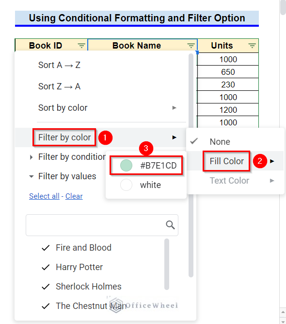
- Click on the filter icon of Column C.
- From the pop-up options, select Filter by Color and then Fill Color. After that, click on #B7E1CD (the color of the formatted cells).
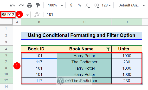
- As you can see, only the duplicated rows are visible. Select the rows.
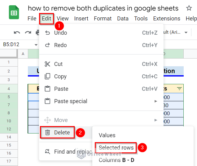
- Go to the Edit ribbon and select the Delete option from there. Then click on the Selected Rows option.
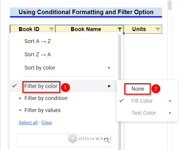
- Thus we have removed all the duplicated rows now. Click on the filter icon of Column C.
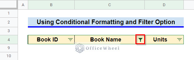
- From the pop-up options, select Filter by Color, and finally, click on None.
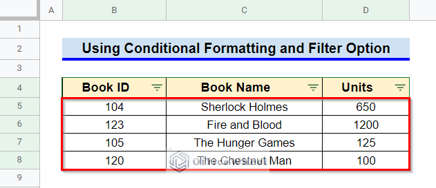
- As you can see, only the rows that were not duplicated remain in the datasheet.
Read More: Google Sheets Use Filter to Remove Duplicates in Column
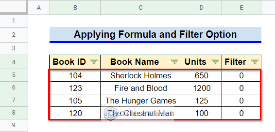
2. Applying Formula and Filter Option
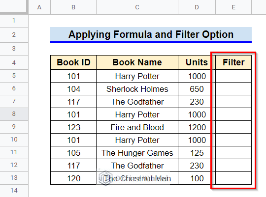
We can combine IF and COUNTIF functions to identify the rows which have been duplicated and then use Filter options to remove all the duplicate rows. For this method, we have to add another column titled Filter to our datasheet.
Steps:
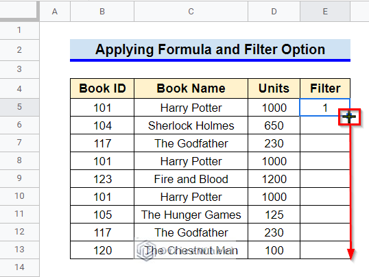
- Select Cell E5 and type in the following formula. Press the Enter key.
=IF(COUNTIF($B5:$B13,B5)=1,0,1)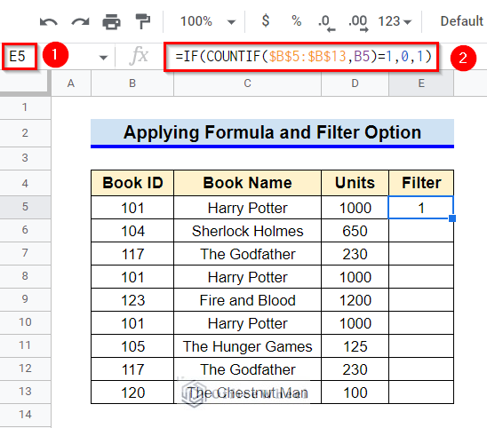
Formula Breakdown
- COUNTIF($B5:$B13,B5)
First, the number of times the value in Cell B5 that is repeated in array B5:B13 is returned by the COUNTIF function.
- IF(COUNTIF($B5:$B13,B5)=1,0,1)
After that, if the return value from the COUNTIF function is equal to 1, the IF function sets the value of Cell E5 as 0 and as 1 if otherwise.
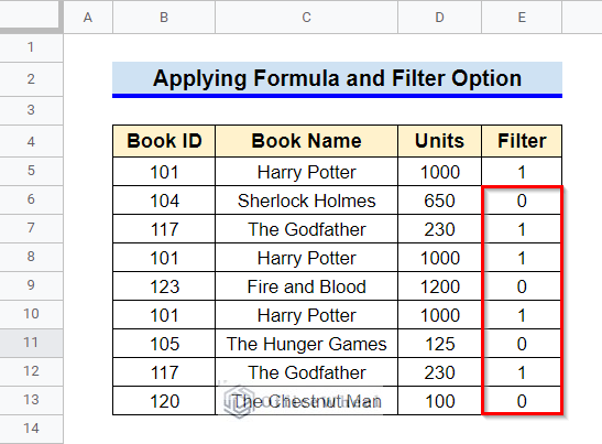
- Select Cell E5 and use the Fill Handle icon to copy the formula into other cells of Column E.
- We have set a filter value of 1 for all the duplicated rows and 0 for all other rows.
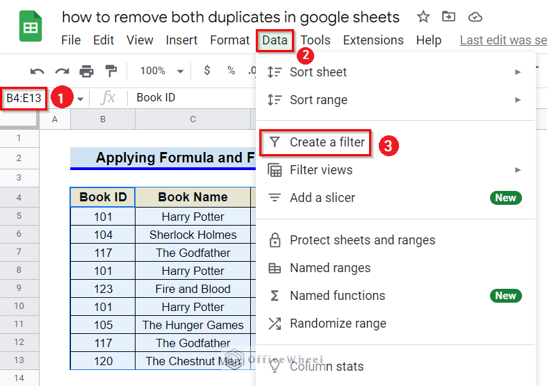
- Select all the cells and then go to the Data Click on Create a Filter from there.
- Click on the filter icon of Column E.
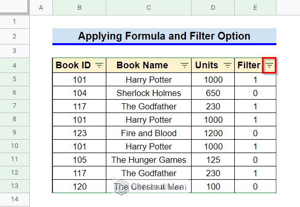
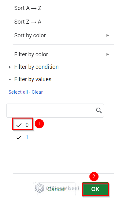
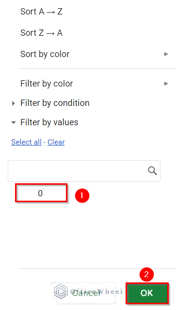
- From the pop-up options, deselect 0 and then click on OK.
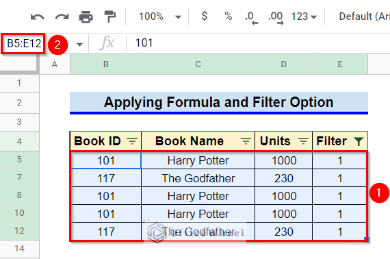
- Only the duplicated rows are visible now. Select the rows.
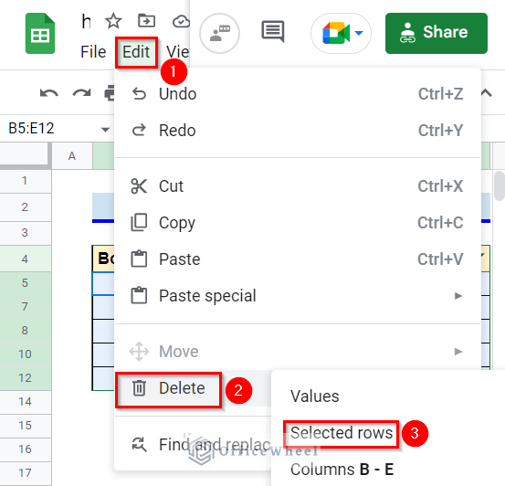
- Go to the Edit ribbon and select the Delete option from there. Then click on the Selected Rows option.
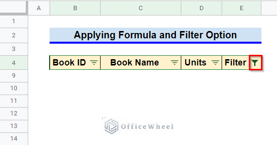
- Thus, we have removed all duplicated rows. Click on the filter icon of Column E.
- Now, from the pop-up options, select 0 and then click on OK.
- As you can see, only rows that were not duplicated remain.
Read More: How to Remove Duplicates in a Column in Google Sheets (5 Ways)
Things to Be Considered
- You must fix the first cell using the $ symbol while entering Range for Custom Formula for Conditional Formatting.
Conclusion
This concludes our article to learn how to remove both duplicates in Google Sheets. I hope that the demonstrated process was sufficient for your requirement. Feel free to leave your thought on the article in the comment section.