Today’s guide focuses on how we can calculate days between dates in Google Sheets. While it is fundamentally simple, Google Sheets allows us to customize this calculation with some of the functions it has on offer made for various scenarios.
How do you calculate days between two dates in Google Sheets?
Primarily, Google Sheets views date as an integer value, starting from 12/31/1899 which has a value of 1. While today’s date, which is 5/16/2022 at the time of writing, has a value of 44697. These date values can be easily extracted by using the DATEVALUE function.
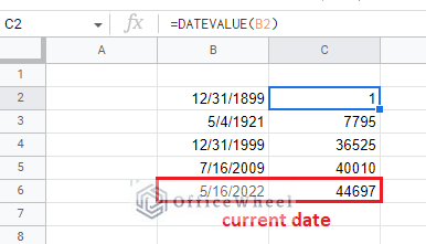
What this means is that every single day has its own integer value. This makes day calculations that much easier.
Now, to calculate the number of days between two dates, we simply have to apply arithmetic subtraction of the dates.
=end_date-start_date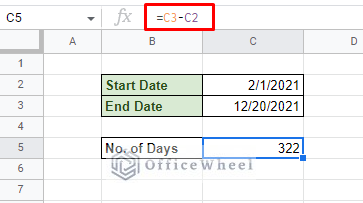
A point to note is that the end_date always has a higher value than the start_date. Thus, it is good to be cautious when inputting these values unless you want a negative date value outcome.
Note: The best way to input date values is to use cell reference as Google Sheets only extracts the underlying value this way. Directly inputting the date will only result in an error or a wrong output. Alternatively, you can use the DATE function to input date values in their respective fields.
More Approaches to Calculate Days Between Dates in Google Sheets
1. Using the MINUS function to find the Difference between Two Dates
Our first method is a direct alternative to the arithmetic subtraction, the MINUS function of Google Sheets. This allows us to encapsulate our date values within a function instead of leaving them out in the open.
While minus is made for simple subtraction, it can be utilized with date values:
To calculate days between dates in Google Sheets using the MINUS function:
=MINUS(C3,C2)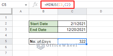
2. DAYS function
Google Sheets provides us with a function explicitly made to calculate the number of days between two dates in a worksheet, that is the DAYS function.
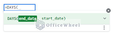
If you were to specialize the MINUS function to only calculate the difference between dates, DAYS is what you would get.
The DAYS function in action:
=DAYS(C3,C2)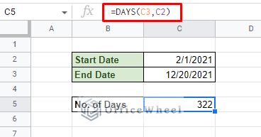
3. Calculating the Number of Workdays Between Dates in Google Sheets
The most common practical use of counting days between dates is when we are counting the effective work days or business days. Once again, Google Sheets has the perfect function for such cases, the NETWORKDAYS function.
NETWORKDAYS(start_date, end_date, [holidays])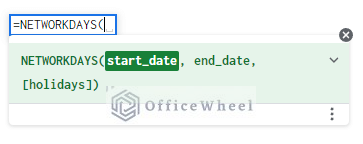
The NETWORKDAYS function counts all the weekdays excluding Saturdays and Sundays (the common western weekend format) between two dates in Google Sheets.
Here we compare the regular day count versus the count performed by NETWORKDAYS:
=NETWORKDAYS(C2,C3)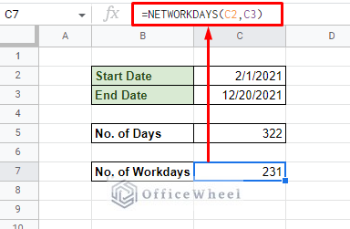
The result with NETWORKDAYS is clearly lower than the regular DAYS count, as expected.
Another point to note is the input format of this function. NETWORKDAYS is the first date function on our list that has the start date ahead of the end date.
But what if the weekends of your region or organization are not Saturdays or Sundays?
For that, we have the slightly more customizable NETWORKDAYS.INTL function.
NETWORKDAYS.INTL(start_date, end_date, [weekend], [holidays])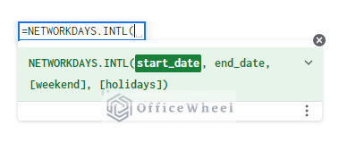
The [weekend] field is where the magic happens. We can determine the weekend combination with a number here. The list of integers and their respective weekends are:
- 1 (default): Saturday and Sunday
- 2: Sunday and Monday
- 3: Monday and Tuesday
- 4: Tuesday and Wednesday
- 5: Wednesday and Thursday
- 6: Thursday and Friday
- 7: Friday and Saturday
Thus, our workday count looks like this with Sunday/Monday weekends:
=NETWORKDAYS.INTL(C2,C3,2)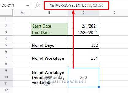
However, the capabilities of the functions don’t end here. Let’s see a couple more examples of the customizability of NETWORKDAYS.
Calculating the Number of Workdays Excluding Public Holidays Between Dates
You may be wondering what the [holiday] field does in the NETWORKDAYS function? We will discuss its use now.
With the [holiday] field you can add a list of dates to exclude from the day count with the function. It could be national, official, or personal days that need to be omitted from the calculation.
The best way to go about it is to make a separate table of holidays and then extract the values from there with cell range reference.
=NETWORKDAYS(C2,C3,$F$3:$F$8)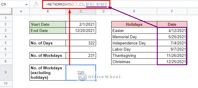
Calculate Custom Workdays Between Dates in Google Sheets
One of the biggest advantages that NETWORKDAYS.INTL has is its weekend, and in turn, weekday customizability.
The [weekend] field of the function can also take a set of specific string values to determine which days to include in the count.
The string must include 7 binary digits (0 or 1) representing each day of the week. This string will of course be inside quotes (“”). E.g., “0011100”.
Here, the first digit of the string represents Monday, and the last digit is Sunday. So, if a workplace only has their workdays fixed to only Mondays, Tuesdays, and Thursdays, our formula will look something like this:
=NETWORKDAYS.INTL(C2,C3,"1101000")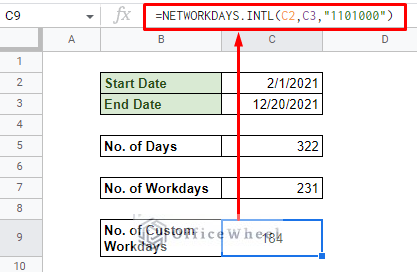
4. DATEDIF Function
DATEDIF is another commonly used date difference calculator on Google Sheets. Where NETWORKDAYS focuses and specializes in workdays and only days, DATEDIF specializes in finding the difference between two dates in Google Sheets with different types of output units, not just days.
DATEDIF(start_date, end_date, unit)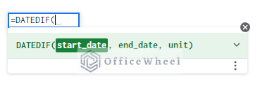
The DATEDIF function works with months, years, and other forms of units that may be useful for date difference calculation. Since we are focusing on only days, the unit field of the function will be “D”.
Our formula:
=DATEDIF(C2,C3,"D")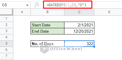
Learn More: Use DATEDIF from Today in Google Sheets (An Easy Guide)
5. DAYS360 Function
The DAYS360 function is a unique way to calculate the number of days between two dates in Google Sheets. The function counts a complete year to have 360 days (30×12 days). This format of a year is often used in some financial calculations.
DAYS360(start_date, end_date, [method])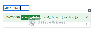
By default, the function uses the US version of the 360-day calendar. But if you want to use the European version, you must set the [method] field to TRUE.
=DAYS360(C2,C3)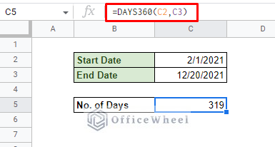
Final Words
That concludes all the ways we can use to calculate days between dates in Google Sheets. While simple arithmetic subtraction can work in most cases, for more customization, you can always look to specialized date functions like NETWORKDAYS and DATEDIF.
Feel free to leave any queries or advice you might have for us in the comments section below.