Combining the VLOOKUP function with the IF statement is sometimes required if you want to look for specific values or data in Google Sheets. In this article, we will show how to use VLOOKUP with an IF statement in Google Sheets easily and effectively.
A Sample of Practice Spreadsheet
Download this spreadsheet to practice yourself.
2 Examples of Using VLOOKUP with IF Statement in Google Sheets
VLOOKUP means vertical lookup. VLOOKUP lets you look for a particular value down the first column in a range of cells. This is what the formula looks like in Google Sheets:
VLOOKUP(search_key, range, index, [is_sorted])IF function in Google Sheets is used to check a condition and then based on it, returns a value if the condition is TRUE, or else returns another value if the condition is FALSE. This is what the formula looks like in Google Sheets:
IF(logical_expression, value_if_true, value_if_false)1. Performing Lookup from Two or More Tables
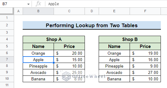
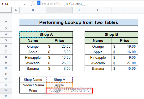
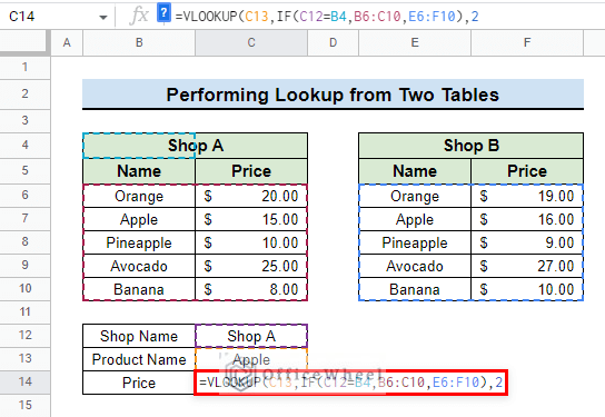
The VLOOKUP function can be used with the IF function to fetch data from 2 different tables. We have a dataset with two tables of two different shops named Shop A and Shop B. We will use the VLOOKUP function along with the IF function to return the Price of Apple from these two tables.
Steps:
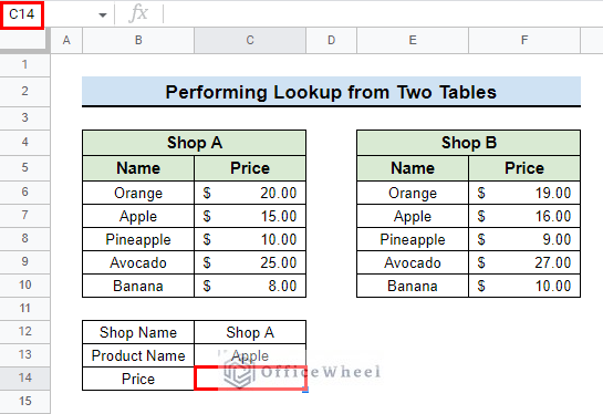
- First, go to the cell where you want to return data. In our example, we go to cell C14.
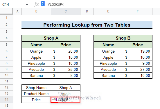
- Then, insert the VLOOKUP function.
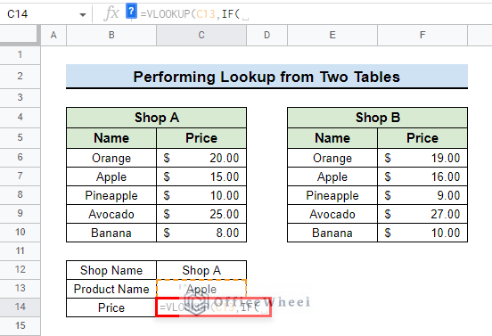
- After that, insert the value that you want to look for followed by a Comma. We kept the value that we want to look for in a different cell. So we type C13.
- Now, Insert the IF function.
- Next, input the logical expression based on which the IF function will return the value. We kept the shop names in n a separate cell to easily formulate the formula. So, we type C12=B4 as we want to match the shop names and return the value if it finds a match.
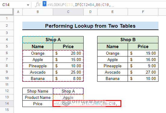
- Then, type the value that you want to show if the IF function finds a match. We want the IF function to return data from range B6:C10 if the value in cell C12 matches the value in cell B4, so we type B6:C10.
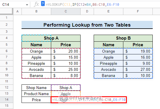
- After that, type the value that you want to show if the IF function does not find a match. We want the IF function to return data from range E6:F10 if the value in cell C12 does not match the value in cell B4, so we type E6:F10.
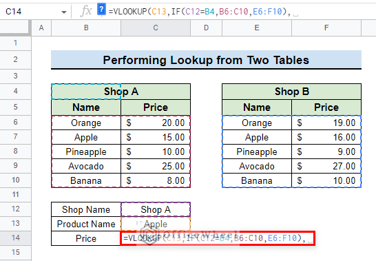
- Then, close parentheses for the IF function followed by a Comma to separate the two functions.
- After that, input the column number from which we want the VLOOKUP to fetch data if the IF function finds a match. We type 2 as the data we want to return is in column 2 of the data table.
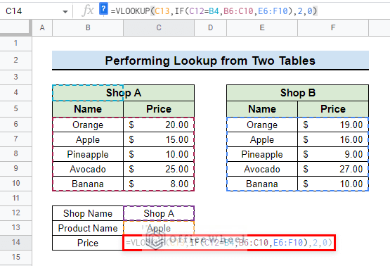
- Then, type 0 or FALSE to get an exact match.
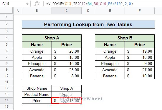
- This is how the final formula looks:
=VLOOKUP(C13,IF(C12=B4,B6:C10,E6:F10),2,0)- Finally, press ENTER to show the value of Apple from Shop A.
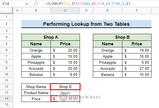
- You can look for the price of Apple from Shop B by simply changing the shop name to Shop B in cell C12.
Read More: How to VLOOKUP Between Two Google Sheets (2 Ideal Examples)
Similar Readings
- How to Concatenate with VLOOKUP in Google Sheets
- Do Reverse VLOOKUP in Google Sheets (4 Useful Ways)
- How to Use VLOOKUP with IF Statement in Google Sheets
- VLOOKUP Multiple Columns in Google Sheets (3 Ways)
2. Using Comparison Operators
Comparison operators such as Greater than (>) and Less than (<) can be used with the VLOOKUP function and the IF function to show some TRUE or FALSE results.
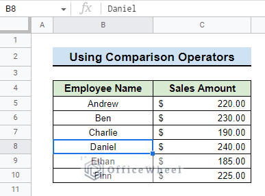
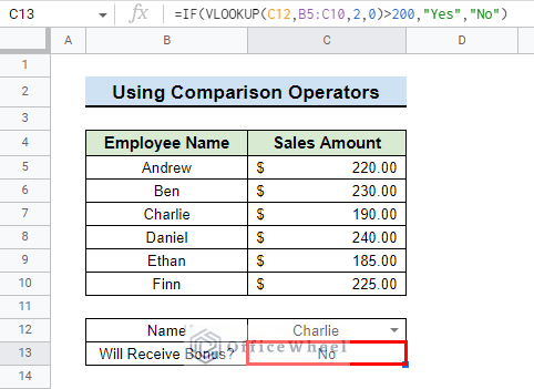
We have a dataset with Employee Name and their Sales Amount. If any one of the employees made a sale of more than $200 then, he will receive a bonus. We will use the IF function with the VLOOKUP to show if Daniel will receive a bonus or not.
Steps:
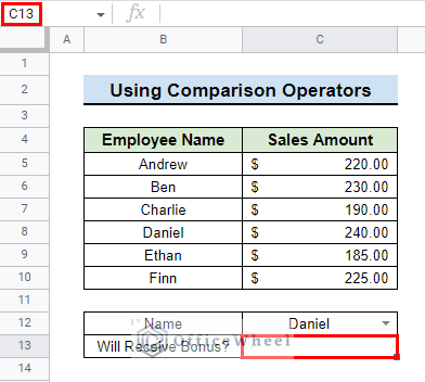
- First, go to the cell where you want to show the result. For our example, we go to cell C13.
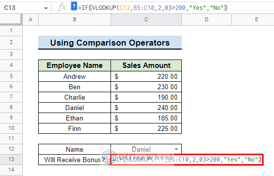
- Then, type in the following formula:
=IF(VLOOKUP(C12,B5:C10,2,0)>200,"Yes","No")Formula Explanation:
- C12 is the data that we want to match with the VLOOKUP The data in cell C13 is Daniel as we have created a Drop-Down list in cell C13 with the Employee Names.
- B5:C10 is the range of the table where the data we are looking up is located.
- 2 is the column number of the data that we want the VLOOKUP to return if it finds a match.
- 0 is used because we want an exact match for the data. You can even use FALSE instead of 0.
- >200 is the condition for the IF function based on which the IF function will return data.
- “Yes” is the text we want the IF function to show if the value we looked up is greater than 200.
- “No” is the text we want to show if the value is not greater than 200.
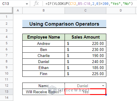
- Finally, press ENTER to show the result. We can see that Daniel made a sale of more than $200, so he will receive a bonus.
- We can select another employee from the drop-down list and check if he will receive a bonus or not. We select Charlie and see that he will not receive a bonus.
Read More: How to Use VLOOKUP with Drop Down List in Google Sheets
Conclusion
In this article, we showed you how to use the VLOOKUP function with an IF statement in Google Sheets with two different examples. Keep practicing the examples that we have shown here for a better understanding of the concept. We hope this article was useful to you to help you.
Also, check out other articles on OfficeWheel to keep on improving your Google Sheets work knowledge.
Related Articles
- How to Use Nested VLOOKUP in Google Sheets
- [Fixed!] Google Sheets If VLOOKUP Not Found (3 Suitable Solutions)
- How to VLOOKUP Between Two Google Sheets (2 Ideal Examples)
- Create Hyperlink to VLOOKUP Cell in Multiple Rows in Google Sheets
- How to Use IFERROR with VLOOKUP Function in Google Sheets
- Use VLOOKUP to Import from Another Workbook in Google Sheets
- How to VLOOKUP Last Match in Google Sheets (5 Simple Ways)
- Use VLOOKUP for Conditional Formatting in Google Sheets

