Knowing how to merge columns in Google Sheets is a fairly easy affair. But things can get complicated when a lot of data and specific criteria are involved.
In this article, we will be covering all the ways you can approach merging your columns in any Google Sheets spreadsheet, no matter the requirements.
Let’s get started.
2 Ways to Merge Columns in Google Sheets
1. Merge Columns using Toolbar Function
We start with the basic merge function of Google Sheets, in other words, the Merge cells option from the Toolbar menu. Which you can find here:
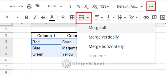
Or here:
Format tab > Merge cells
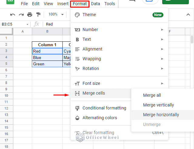
Since we are working on merging columns only, we will be using the Merge horizontally function.
Data Loss
When we click on Merge horizontally, we are hit with the following warning:
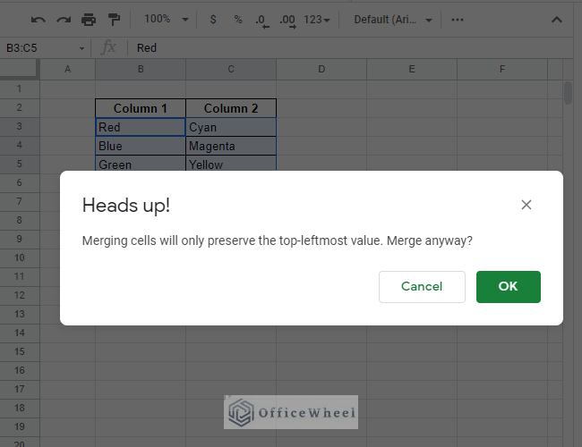
It simply means that, if we go forward with merging our selected cells, some of the values may get overwritten as a result of merging horizontally.
Our result after clicking OK:
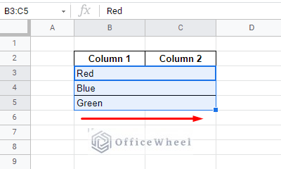
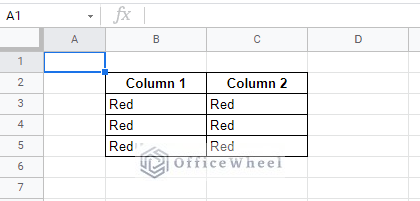
As we can see, the cell merge happed towards the right along with the columns. The data in Column 1 remained but has overwritten the data in Column 2.
This, unfortunately, will always happen every time we merge cells, columns, or rows in Google Sheets.
But what happens if we merge columns that contain the same data?
We have now organized our columns with the same data.
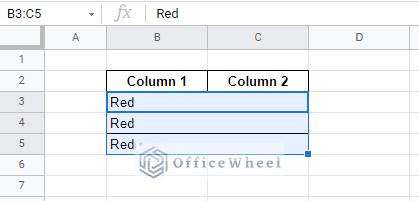
Clicking on Merge horizontally again prompts a warning, and our result is as expected.
If you want to retain the data in the cells, we have a few workarounds for you in the next section.
2. Combine Columns with Formula
The best way to combine or merge data from different columns is to use functions in Google Sheets. Here, you won’t be directly merging in position, but the combination will happen in a separate cell.
We have two ways to combine data from different columns with formulas in Google Sheets:
- Horizontally
- Vertically
A. Combine Columns Horizontally in Google Sheets
To show our horizontal combination methods, we have created the following worksheet.
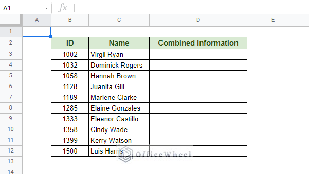
Here, we will be combining the data from the ID and Name columns into the Combined Information column with a hyphen (-) separator.
I. Ampersand (&) Operator
We start off simple by using the concatenate operator in Google Sheets, the ampersand operator (&). This operator will help us combine two or more cell references and other data together in one cell.
Our formula at D3:
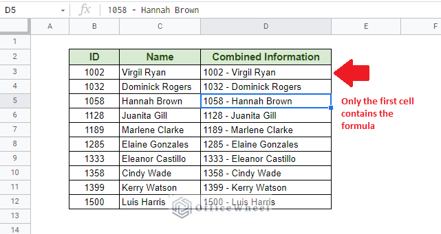
=B3&" - "&C3You can use the fill handle to apply the formula to the rest of the column.
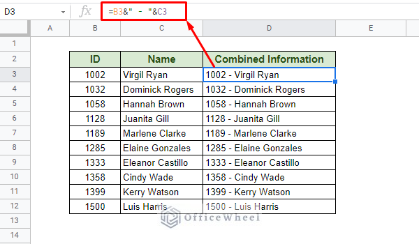
As you can see, different fragments of our data have been concatenated together using the ampersand (&) operator between them.
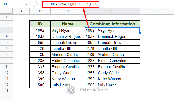
II. CONCATENATE Function
Speaking of concatenating, we can also use the CONCATENATE function of Google Sheets to achieve the same results.
Our formula:
=CONCATENATE(B3," - ",C3)You can use the fill handle to apply the formula to the rest of the column.
If you are only looking to combine two columns, as we see here, you can keep things simple by using the CONCAT function instead. The formula will be:
=CONCAT(B3&" - ",C3)CONCAT only takes two string values, thus we have to use the & operator with the first cell reference to add the hyphen (-).
III. Combine With Line Break
Next, we will be working with the following worksheet.
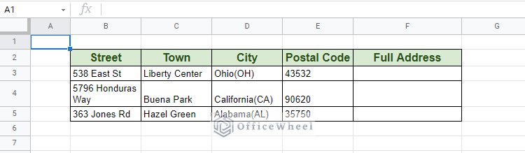
As before, we are looking to combine all the data in the different columns into one cell. But this time, we will be adding data with a line break instead of a hyphen (-) or a comma (,) separator.
The formula or code for a line break in Google Sheets is CHAR(10). We will be adding this to our ampersand formula.
=B3&CHAR(10)&C3&CHAR(10)&D3&CHAR(10)&E3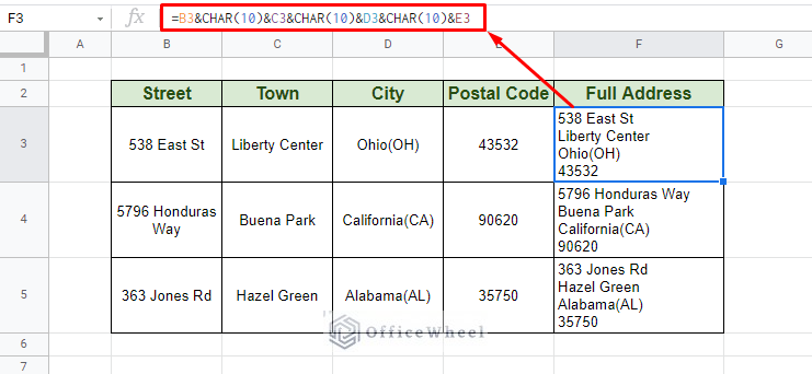
We can create a more automated version of this formula, given that all of our columns are adjacent, by using the TEXTJOIN function:
=TEXTJOIN(CHAR(10),,B3:E3)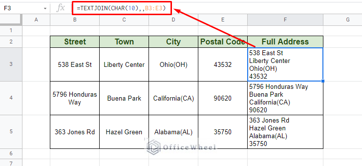
IV. Using an Array
The final method we will be discussing for this section involves a process to automate the concatenate formulas.
Here, we will be adding the column range instead of individual cells to the formula. This will make it an array formula, which in turn means that we have to use the ARRAYFORMULA function to make it work.
Our column ranges:
B3:B12 and C3:C12
Therefore, our new formula:
=ARRAYFORMULA(B3:B12&" - "&C3:C12)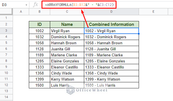
The advantage of using this formula is that you do not have to individually input the formula in each cell of the column. It automatically pulls the data and displays them in one go.
You can also use the CONCAT function version of the formula as well. Simply replace the formula inside the ARRAYFORMULA with the CONCAT formula:
=ARRAYFORMULA(CONCAT(B3:B12&" - ",C3:C12))B. Combine Columns Vertically in Google Sheets – Making a List
Columns are not confined to horizontal merges, we can merge them vertically as well, thanks to Google Sheets formulas.
Combining columns vertically simply means adding them on a separate column as a list. For that, we will be using the following worksheet.
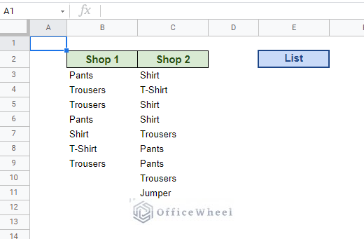
I. Using Arrays
We start this time with arrays directly. Another unique feature of the formula that we are going to be showing is that it uses a semicolon (;) separator instead of a comma (,) separator.
Let’s create our formula.
Step 1: Start off with an equals-to and open a curly brace, ={
Step 2: Input the range of the first column. In our case it is B3:B11.
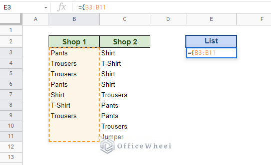
Step 3: Input a semicolon (;), this will tell the spreadsheet to continue adding data along the same column it is in currently.
Step 4: Input the range of our second column, C3:C11.
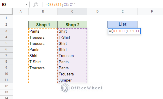
Step 5: Close curly braces and press Enter.
Our final formula:
={B3:B11;C3:C11}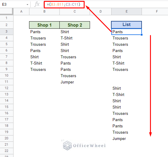
Notice that the blank cells from the first column are also included in our list, that is because we have included them in our range, B3:B11. This only means that the array takes everything into account.
To remove blank cells, you can simply remove them from the range, B3:B9. Or read further to read about some modifications to the formula that will ignore them.
II. Using the UNIQUE function to remove duplicates
As you have seen, there are a lot of duplicates on our list. To remove these duplicates, we simply utilize the UNIQUE function.
Just enclose the previous formula within the UNIQUE function:
=UNIQUE({B3:B11;C3:C11})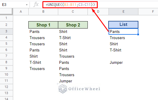
Read More: How to Use Formula to Highlight Duplicates in Google Sheets
III. Using the FILTER and LEN functions to remove blank cells
Now let’s see if we can do something about those blank cells. To do that, we will be taking the help of two Google Sheets functions, FILTER and LEN.
Our formula:
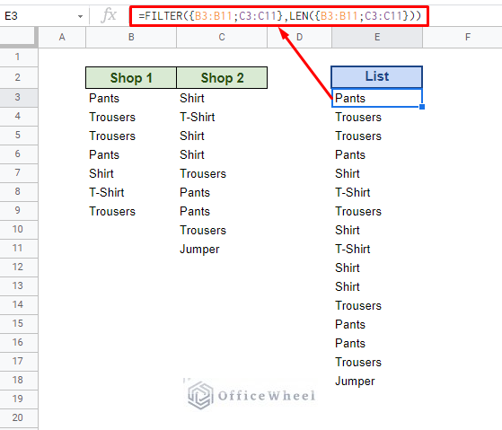
Formula Breakdown:
- {B3:B11;C3:C11}: Our array range. You can also use {B3:B;C3:C} if you want to make your list more dynamic.
- LEN({B3:B11;C3:C11}): Acts as the condition for the FILTER function. Checks if the cell is not empty.
- FILTER: Extracts the values from the range according to the set conditions.
You can even slap in the UNIQUE function over it to extract only unique values without blank cells.
=UNIQUE(FILTER({B3:B11;C3:C11},LEN({B3:B11;C3:C11})))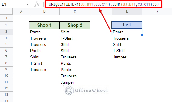
IV. Merge two different categories of columns
Our final process is a bit niche. We will be looking to list all of the sales achieved by each seller. As you can understand, this process helps us list by category.
We will be going over it step-by-step.
Step 1: We will count the categories (Name) first. We input the formula:
=ARRAYFORMULA(COUNTIFS(B3:B,B3:B,ROW(B3:B),"<="&ROW(B3:B)))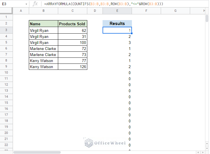
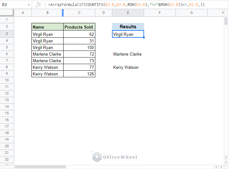
Step 2: We will add an IF condition to replace duplicates with blanks. The syntax for this step is:
ArrayFormula(if(formula-from-step-1=1,B3:B,))Our formula:
Step 3: We will finally merge the two columns into one. For this, we will be using the FLATTEN function.
We will enclose our previous formula with FLATTEN and curly braces, like so:
FLATTEN({ArrayFormula(if(COUNTIFS(B3:B,B3:B,ROW(B3:B),"<="&ROW(B3:B))=1,B3:B,)),C3:C})***DO NOT input this formula in your worksheet just yet. Inputting this formula will make your spreadsheet go on an infinite loop, perhaps even crashing your browser!
We will now add our newfound formula to the following syntax:
FILTER(step 3 formula, step 3 formula<>"")To get our final formula:
FILTER(FLATTEN({ArrayFormula(if(COUNTIFS(B3:B,B3:B,ROW(B3:B),"<="&ROW(B3:B))=1,B3:B,)),C3:C}), FLATTEN({ArrayFormula(if(COUNTIFS(B3:B,B3:B,ROW(B3:B),"<="&ROW(B3:B))=1,B3:B,)),C3:C})<>"")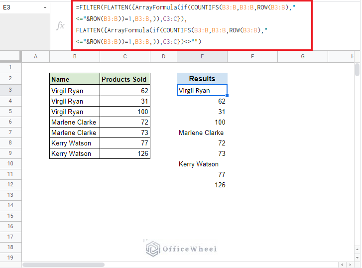
Note: We have left our ranges open-ended, B3:B, in case more column values are added in the future. You can limit the range, B3:B9, as well to avoid infinite loop errors as we warned you about in Step 3.
The formula combinations for the merge of columns don’t end here. You can take it upon yourself to customize these formulas we have discussed and create one that suits your spreadsheet.
Final Words
While merging cells is a piece of cake in every spreadsheet application, making more specific merges with desired conditions, like we have discussed in this article, takes a bit more working knowledge.
We hope that this article is able to make you understand how to merge columns in Google Sheets, as well as give you an insight into the complexities that arise when we want merges that cater to some complex criteria. However, if you want to know only the general idea behind merging cells, please have a look at our How to Merge Cells in Google Sheets article.
Please feel free to leave any queries or advice in the comments section below.