How to Merge Cells In Google Sheets Without Losing Data

Sometimes, the traditional ways to merge cells in google sheets may not cut it, thanks to the wiping of data that happens with the built-in function.

For these reasons, we have to get a little creative with the functions, formulas, and add-ons available to us.

In this article, we will be discussing in-depth these processes to merge cells in Google Sheets without losing data.

Let’s get started.

5 Ways to Merge Cells Without Losing Data in Google Sheets

1. Using the Ampersand (&) Operator

The simplest way to merge data from multiple cells into one cell is by using the ampersand operator (&).

What it does is a no-brainer, placing it between two values concatenates them together.

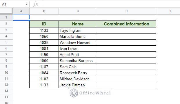
In the following worksheet, we will combine the values of the ID and Name columns into the Combined Information column with the help of the & operator.

We type in the following formula in cell D3:

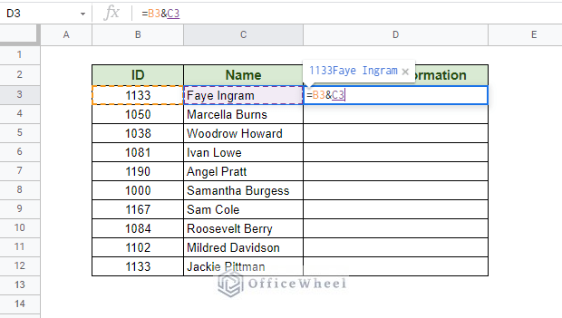
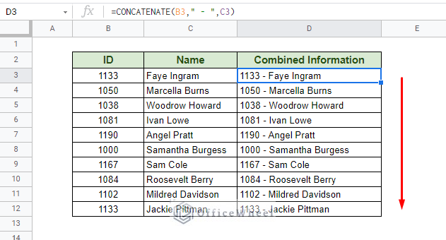
Use the fill handle to apply the formula to the rest of the column.

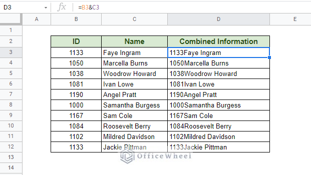
This merge of the data is not very presentable. So, let’s add a separator in-between the data to make it so.

Adding a Separator

Remember that a separator is usually in Text format and that they are a separate piece of data, so we have to enclose them in quotation marks (“”) and insert the ampersand operator on either end.

Our modified formula with whitespace:

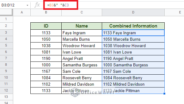
Our modified formula with hyphen (-):

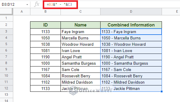
Adding Line Breaks

We can also add line breaks to our combination. The function or code for adding line-breaks is CHAR(10). We simply replace the hyphen separator with it:

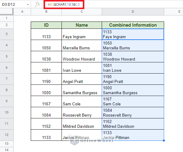
2. Using the CONCATENATE Function

The CONCATENATE function can act as a direct alternative to the ampersand operator method.

The syntax:

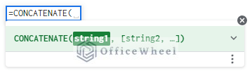
Here, we can individually add data values or text within the function, separated by commas (,).

Let’s apply it to our worksheet:

Step 1: Input =CONCATENATE( in cell D3.

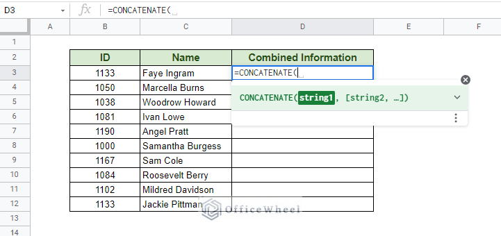
Step 2: Input the cell references to the values you want to combine. In our case, it is B3 and C3. Do not forget to add the separator in between the values, “ – “.

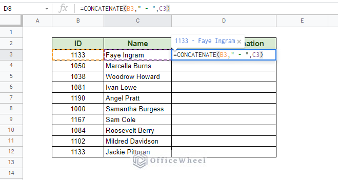
Step 3: Close parentheses and press ENTER. Apply the formula to the rest of the column.

Note: You can replace the “ – “ with CHAR(10) to add a line break as a separator instead.

If you only have two values to concatenate, as we have seen in our worksheet, you can also use the CONCAT function to get things done.

With separator:

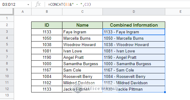
3. Using the TEXTJOIN Function

TEXTJOIN is the second function that we will be using to merge values from different cells.

The syntax:

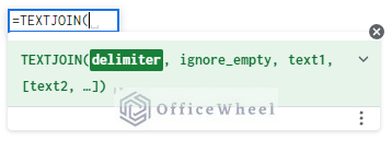
Breakdown:

• delimiter: What our separator will be.
• ignore_empty: Takes a Boolean value on whether the function should ignore empty cells or not.
• text1, [text2, …]: Our data, cell values or reference.

We will be using the following worksheet to show our TEXTJOIN example:

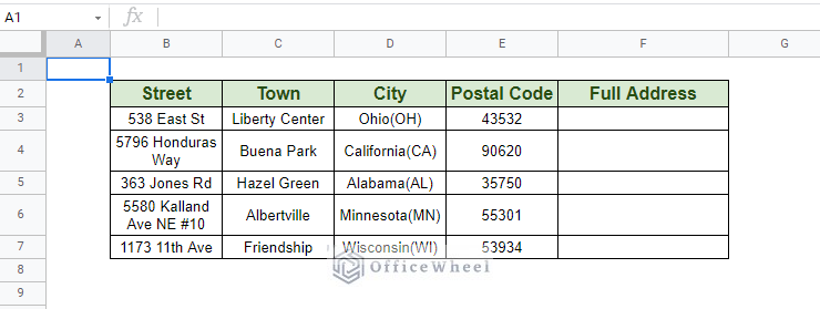
We will be looking to merge all the separate pieces of the addresses into one cell separated by commas.

With that, our TEXTJOIN formula to merge cell values will be:

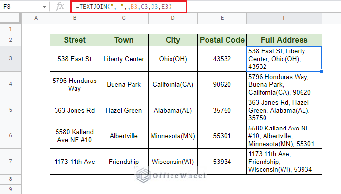
You can also put your values in as a range:

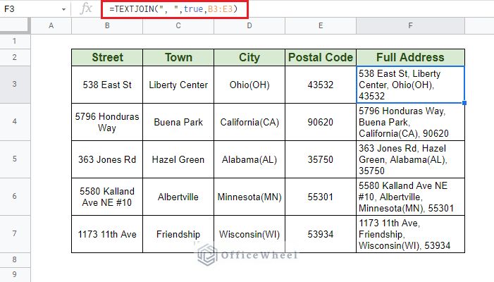
Note that we have left the ignore_empty section of the function as TRUE. We want to ignore any empty cells that may be included in our range of values.

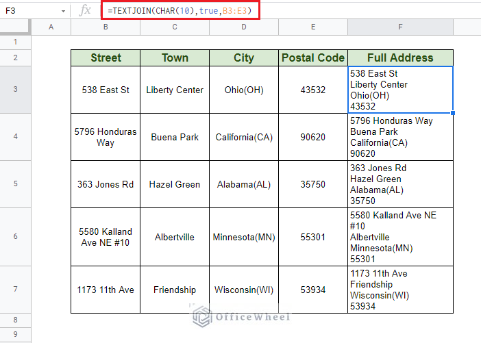
Adding Line-Breaks

To add line-breaks, simply replace the delimiter value with CHAR(10):

4. Merging Different Variable Types (Numbers and Text)

For this section, we will be using the following dataset:

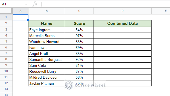
Notice that we have two types of variables, one is your regular text (Name) and the other is in a number format (Score), namely in the percentage format.

What do you think happens when we apply one of our previously shown methods to combine these column values?

Let’s see:

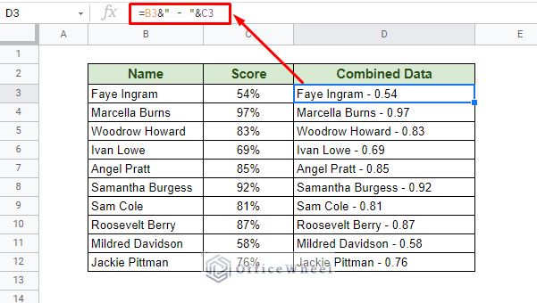
The percentage number format is not being carried over.

Google Sheets views its values in cells in its base form (54% is 0.54 numerically), that base form is being carried over.

To remedy this, we must make some changes. We have to transform the value into something that reflects the format it is currently in. The best way to do this is by utilizing the TEXT function.

We will incorporate the percentage value as text using the TEXT function:

• C3 is our target cell.
• # represents the wildcard symbol for the number.
• The % symbol will be added as a text after the number

Combining with our original formula:

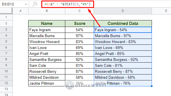
A version for Dates

Another common number format in spreadsheets is the date.

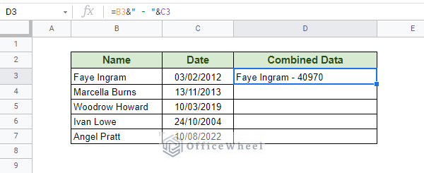
As you can see, the date has transformed back to its base numerical value.

We, once again, take the same approach. But this time, we have to change our formatting to match that of a date within the TEXT function. (Default: dd/mm/yyyy)

Combining with our formula:

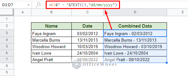
Note: You can replace “dd/mm/yyyy” with any date format that suits your spreadsheet or work.

5. Using an Add-On

We all know that using the default merge of Google Sheets on cells that contain values will give us not so desirable results. In other words, merging cells in this method will only leave behind one cell or only the leftmost results while wiping out all the other ones.

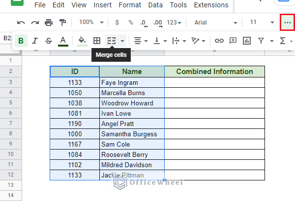
Google Sheets’ built-in Merge option

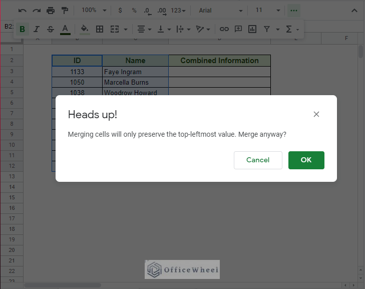
Merge warning prompt

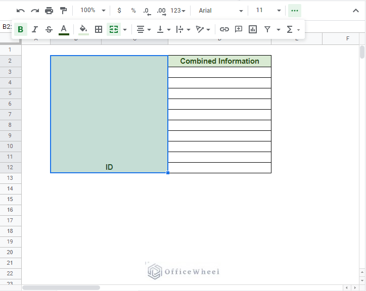
Our not so desirable result from built-in Merge cells function.

To make this Merge function more intuitive and customizable, we have to download an add-on called Merge Values.

To open up the add-ons page, simply navigate: Extensions tab > Add-ons > Get Add-ons

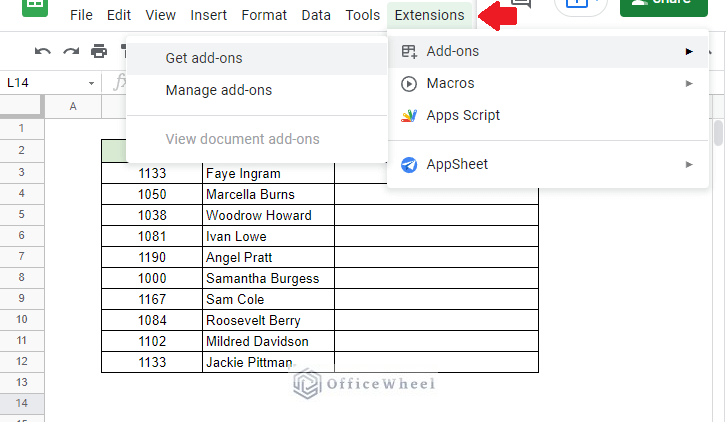
Here, search for the Add-on Merge Values, as shown in the following image:

Download and add it to your Google Sheets. The add-on is free to use and setup will take less than five minutes.

The Step-By-Step Process

Let’s now see how we can merge our ID and Name columns into one using this add-on.

Step 1: Select the cells you want to merge, for us, we have selected the ID and Name columns.

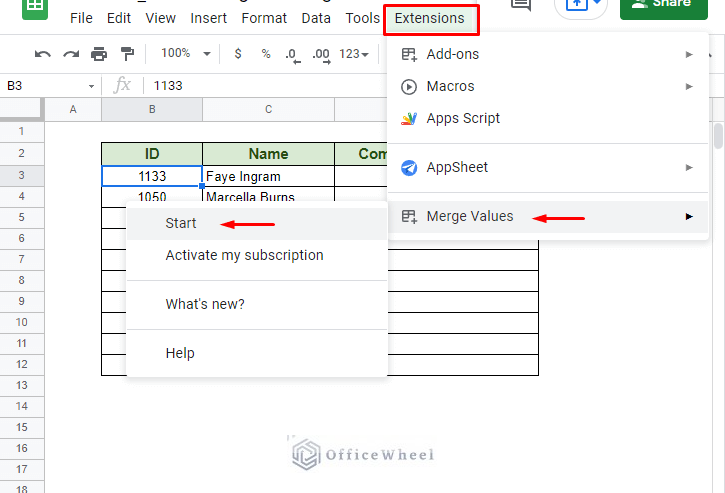
Step 2: Open the Merge Values menu. Extensions tab > Add-ons > Merge Values

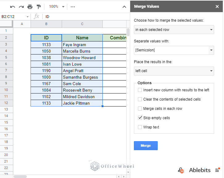
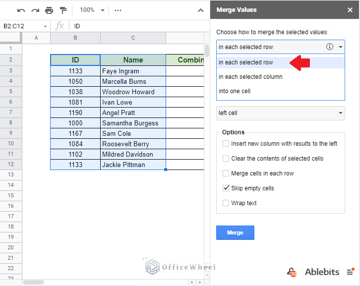
Step 3: For our direction of merge, we will select “in each selected row”.

Note: For row/vertical merge, select the “in each selected column” option.

Step 4: For our delimiter value we select [Space].

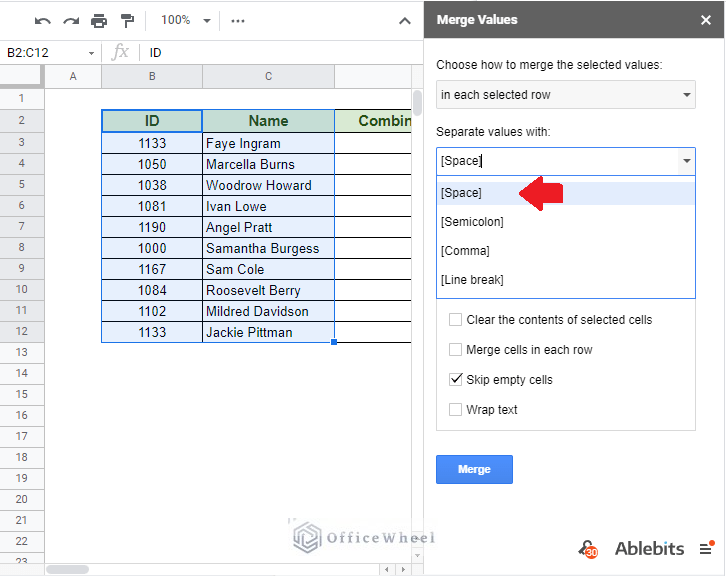
Note: You can add any other iteration of delimiter as well, like [Space]and[Space] or [Space]-[Space].

Step 5: Select the “merge cells in each row” option.

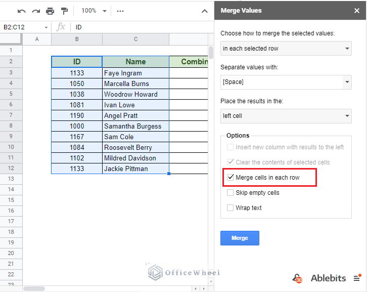
Options Breakdown:

• Insert new column with results to the left: Adds a new column according to the direction of the merge.
• Clear the contents of selected cells: Empties the previous cells after the merge.
• Merge cells in each row: Merges the cells along with the values. Selecting this will gray out the previous two options.
• Skip empty cells: Will only take non-empty cells into account during the merge.
• Wrap text: Will wrap text in cells after merge.

Step 6: Click Merge to finish.

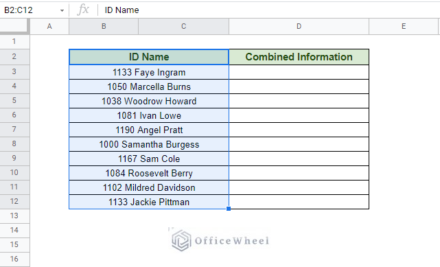
You can perform any formatting you like on the result.

A word of advice: Create a backup of your data before using this add-on, especially if you are a free user, since the add-on does not allow you to roll back changes. Subscribed users will have the option to backup the entire worksheet in the Options menu.

Final Words

We hope that all of the methods we have discussed today can help you ease your way through some of the convoluted merging tasks that you may face while working in Google Sheets. Namely, that of how to merge cells in google sheets without losing data.

Please feel free to leave a comment with any queries or advice you may have for us.

Related Articles

• Unmerge Cells in Google Sheets (4 ways)
• How to Merge Columns in Google Sheets
• How to Merge Rows in Google Sheets (3 Ways)