We frequently use Google Sheets to average or sum any data. When we need to average a dataset that is based on a specific set of criteria, we compute the weighted average. Sometimes we need to calculate the weighted average with some conditions. We can use different Google Sheets functions to do that. In this article, we will demonstrate some methods to calculate the conditional weighted average in Google Sheets.
A Sample of Practice Spreadsheet
You can download the practice spreadsheet from the download button below.
What Is Conditional Weighted Average?
A weighted average is an arithmetic mean that accounts for the relative importance of different data points. It means the average is calculated giving specific data more priority depending on their value or criteria. This gives a more accurate result than the regular arithmetic mean.
And a conditional weighted average is when the weighted average is calculated taking multiple conditions in importance.
5 Suitable Ways to Calculate Conditional Weighted Average in Google Sheets
Here we will show 5 easy and effective ways to calculate the weighted average in Google Sheets.
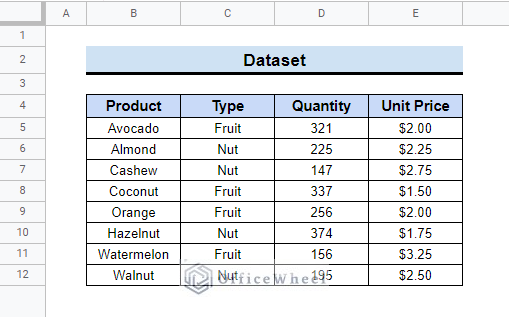
Let’s assume we have a dataset that contains data about 2 types of foods (fruit and nut) and their quantity and unit price. We will perform a conditional weighted average to find out the average unit price of one type of food (fruit).
Here with a few steps, we will show how to calculate the conditional weighted average of unit price. Follow the article to learn how to do that.
1. Applying Generic Formula
A simple generic formula can be used to determine the conditional weighted average. The generic formula is given below.
Weighted Average= (Total of Weighted Terms)/(Total Number of Terms)
The instructions to do that are given below.
📌 Steps:
- First, select cell E13 and enter the below formula.
=(D5*E5+D8*E8+D9*E9+D11*E11)/(D5+D8+D9+D11)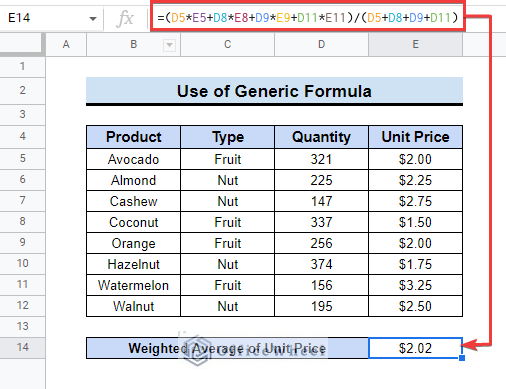
- Here, D5*E5 in the formula returns the product of quantity and unit price of Avocado i.e the 1st fruit in the dataset. So D5*E5+D8*E8+D9*E9+D11*E11 returns the sum product of quantity and unit price for all fruits. So you get the Total Weighted Terms for the Fruit type.
- The quantity is the weighting factor in this dataset. Now D5+D8+D9+D11 returns the sum of the quantities. So you get the Total Number of Terms for the generic formula.
Read More: How to Use Weighted Average Formula in Google Sheets
2. Implementing SUMIFS Function
We can also use the SUMIFS function to find out the weighted average for different conditions. The SUMIFS function returns the sum of a range depending on multiple criteria. This will give output for conditional weighted average. Check the below steps to be able to do that.
📌 Steps:
- First, select F5 and enter the below formula to find the total price of the food product(Avocado). Next, use the fill handle tool to drag down the formula from cell F6 to F12.
=D5*E5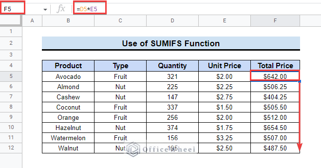
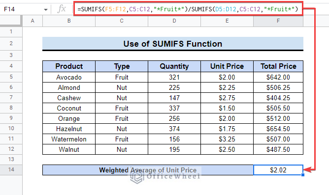
- Then select cell F14 and enter the formula. Next, you will get the result for the weighted average of unit price for the Fruit category. You can get the unit price of nuts by replacing Fruit with Nut in the formula.
=SUMIFS(F5:F12,C5:C12,"*Fruit*")/SUMIFS(D5:D12,C5:C12,"*Fruit*")
Formula Breakdown
- SUMIFS(F5:F12, C5:C12,”*Fruit*”): This formula sums the total price from cell range F5: F12 if they are of the “Fruit” type in cell range C5:C12.
- SUMIFS(D5:D12, C5:C12,”*Fruit*”): This formula sums the quantity from cell range F5: F12 if they are of the “ Fruit” type in cell range C5:C12.
- SUMIFS(F5:F12, C5:C12,”*Fruit*”)/SUMIFS(D5:D1 2, C5:C12,”*Fruit*”): If you divide the total price by quantity, you will get the weighted average of unit price.
3. Applying SUMPRODUCT and SUMIF Functions
Implementing the SUMPRODUCT and SUMIF functions together is another way of calculating the conditional weighted average. The SUMPRODUCT function calculates the sum of the products of two same-sized strings or ranges. The SUMIF function returns a conditional sum across a range. Here we will use these two functions to find out the weighted average. Follow the steps to learn how to do that.
📌 Steps:
- First, select cell E14 to input the below formula.
=SUMPRODUCT((C5:C12="Fruit")*D5:D12*E5:E12)/SUMIF(C5:C12,"Fruit",D5:D12)
- It will provide the result which is the weighted average value for Fruit unit price.
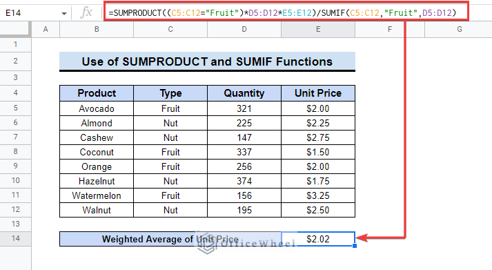
Formula Breakdown
- SUMPRODUCT((C5:C12=”Fruit”)*D5:D12*E5:E12): This function multiplies values from D5:D12 and E5:E12 ranges if they are under fruit type from C5:C12.
- SUMIF(C5:C12, “Fruit”, D5:D12): This function just gives the sum of values from the range D5:D12 if they fall under the Fruit type.
- Finally dividing the output of the SUMPRODUCT function by the output of the SUMIF function gives back the weighted average of the unit price for the fruits.
4. Utilizing AVERAGE.WEIGHTED and FILTER Functions
Google Sheets has a function dedicated to calculating the weighted average. We will use the AVERAGE.WEIGHTED function to calculate the conditional weighted average of unit price in Google Sheets. The AVERAGE.WEIGHTED function returns the weighted average of a set of values, given the values and the corresponding weights. We will also use the FILTER function to find the conditional weighted average of unit price for Fruits. You can follow the steps below to do this by yourself.
📌 Steps:
- First, select cell E14 and enter the formula in the cell.
=AVERAGE.WEIGHTED(FILTER(E5:E12,C5:C12="Fruit"),FILTER(D5:D12,C5:C12="Fruit"))
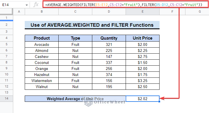
- Here, the FILTER function will return the quantity and unit price for the fruits only. The output of this function will work as arguments of the AVERAGE.WEIGHTED function.
5. Using SUMPRODUCT, ISNUMBER, and SEARCH Functions
Alternatively, we can combine three functions to get the conditional weighted average in Google Sheets. We will use the SUMPRODUCT, ISNUMBER, and SEARCH functions to accomplish that. Read the following steps to do that.
📌 Steps:
- First, select cell E14 and insert the below formula to get the same result as earlier.
=SUMPRODUCT((ISNUMBER(SEARCH("Fruit",C5:C12))*(D5:D12)*(E5:E12)))/SUMPRODUCT((ISNUMBER(SEARCH("Fruit",C5:C12))*(D5:D12)))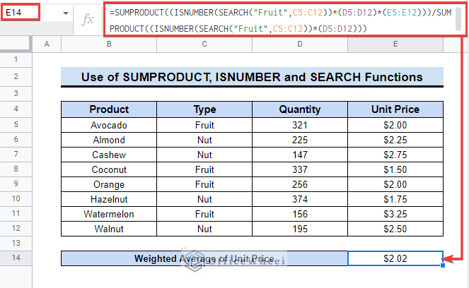
- SEARCH(“Fruit”,C5:C12): The SEARCH function specifies the cells containing “Fruit” in the C5:C12 range.
- ISNUMBER(SEARCH(“Fruit”,C5:C12)): The ISNUMBER function verifies whether the output of the SEARCH function is a number.
- SUMPRODUCT((ISNUMBER(SEARCH(“Fruit”,C5:C12))*(D5:D12)*(E5:E12))): This part returns the Total Weighted Terms for the fruits only.
- SUMPRODUCT((ISNUMBER(SEARCH(“Fruit”,C5:C12))*(D5:D12))): Here the SUMPRODUCT function returns the sum of quantities for fruits only.
Things to Remember
- If you use the AVERAGE.WEIGHTED function, make sure to enter values into every cell; otherwise, the formula will return an error. To avoid this issue put a “0” in blank cells.
Conclusion
Hopefully, the methods above will be enough for you to calculate the conditional weighted average in Google Sheets. You can check the practice spreadsheet and then practice on your own. Please use the comment section below for any further queries or suggestions. You may also visit our OfficeWheel blog to explore more about Google Sheets.