In Google Sheets, sometimes we need to find the lowest number in a row. Highlighting the lowest value helps to visualize or find the data easily. There are some easy methods to highlight the lowest value in a row in Google Sheets. In this article, we will demonstrate how to do this task to make your dataset more understandable.
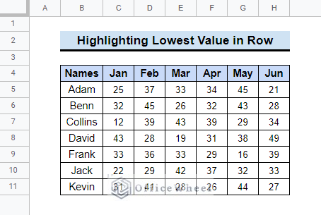
A Sample of Practice Spreadsheet
You can download the practice spreadsheet from the download button below.
2 Easy Ways to Highlight the Lowest Value in a Row in Google Sheets
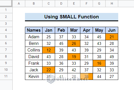
Let’s assume we have a dataset that represents the total miles a person ran in a month for six months. We want to highlight the lowest miles for each person to know in which month he ran the lowest.
Conditional Formatting is a great feature in Google Sheets to format data as required based on conditions. We will use this tool to highlight the lowest value in a row. We will use two functions to do that. Follow the methods below to apply these formulas.
1. Utilizing SMALL Function with Conditional Formatting
We will use the SMALL function to highlight the lowest value. The SMALL function works just like its name, it returns the smallest value from a range of numbers. We will show how to use it to highlight the lowest value in a row in Google Sheets. Follow the steps to be able to do it by yourself.
📌 Steps:
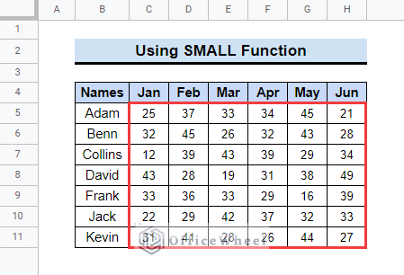
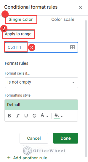
- First, select the range where you want to highlight the lowest values in rows. Here, we set the cell range C5:E11.
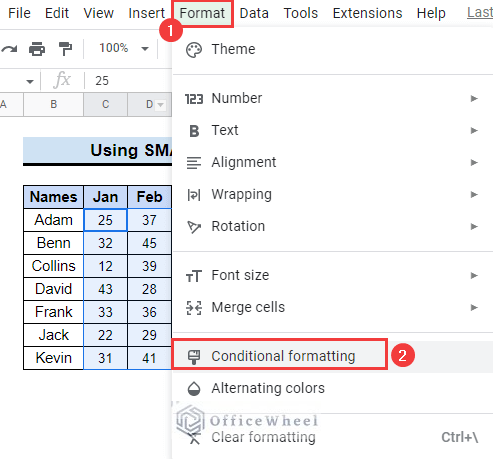
- Then, select the Format option from the menu bar. In the drop-down, you need to click on the Conditional formatting option.
- After that, you will see the Conditional format rules pane on the right side of the page.
- Next, check if you are on the Single color tab. Below that in Apply to range, it will show the range you selected before.
- Then, in Format rules there is a drop-down under the option Format cells if. Choose the “Custom formula is” option from there.
- A box will appear named Value or formula. Insert the following formula in the box.
=C5<=SMALL($C5:$H5,1)- Here the function finds the smallest value from the range C5:H5. And 1 means the 1st lowest value from the row. If you type 2 or 3 after the comma instead of 1, it will also highlight the bottom 2 or 3 values respectively.
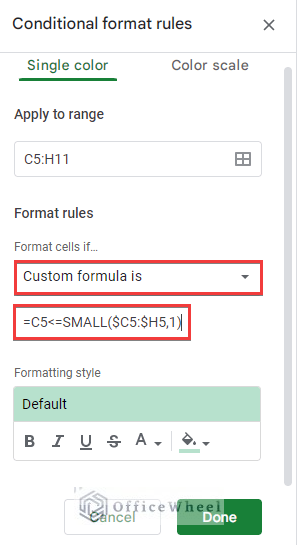
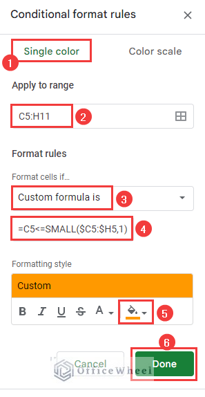
- Now, to highlight the lowest values, select a color from the Fill color option under Formatting styles.
- Finally, after all these steps click on the Done button.
- After applying the Conditional formatting your data table will look like the following image.
Read More: Highlight Row If Cell Contains Text with Conditional Formatting in Google Sheets
Similar Readings
- Highlight Row Based on Date in Google Sheets (2 Suitable Ways)
- How to Highlight Every Other Row in Google Sheets (2 Methods)
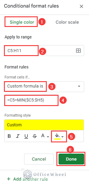
2. Using Conditional Formatting with MIN Function
Alternatively, you can also use the MIN function to highlight the lowest value in a row in Google Sheets. This function returns the minimum value in a numeric dataset. Follow the steps below to apply this function in the Conditional formatting tool in Google Sheets.
📌 Steps:
- This method is also the same as the previous one. This time we will only use another different function to do the same thing.
- First, select the range (C5:H11) and then go to Format >> Conditional formatting.
- All the steps till the Value or formula will be the same as before. Then, enter the following formula in the Value or formula box.
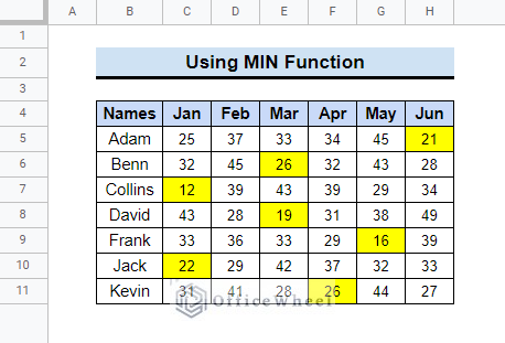
=C5=MIN($C5:$H5)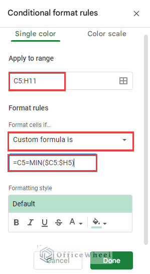
- Then, choose any color from the Fill color option to highlight the lowest values in the row.
- This will show the lowest value in every row highlighted like this image.
Read More: How to Highlight Active Row in Google Sheets (2 Suitable Ways)
How to Highlight the Highest Value in a Row in Google Sheets
You can also highlight the highest value in a row in Google Sheets. You only need to change the formula in Conditional formatting.
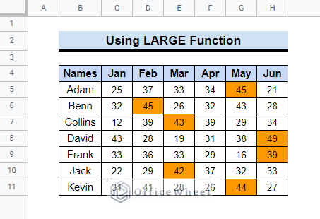
- You can apply the LARGE function to highlight the highest value. This function will return the largest value in the row. Apply the following formula as the conditional formatting rule.
=C5>=LARGE($C5:$H5,1)- After that, you will see the following result.
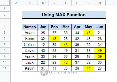
- Alternatively, you can also apply the MAX function to get the highest value. The MAX function returns the maximum value from a set of values. The formula for the conditional formatting rule will be as follows.
=C5=MAX($C5:$H5)- After applying the conditional formatting, you will get the following output.
Read More: How to Highlight Highest Value in Row in Google Sheets (2 Ways)
Things to Remember
- You need to use the cell references in the formulas properly. Otherwise, you may not get the desired results.
- You can also highlight the highest and lowest values in the same row using Add another rule option in Conditional formatting.
Conclusion
We hope now you know how to highlight the lowest value in a row in Google Sheets. Please use the comment section below for further queries or suggestions. Hopefully, it will help you to visualize your data more properly. You may also visit our OfficeWheel blog to explore more about Google Sheets.