We often need to apply different formulas in our calculations in Google Sheets. A large spreadsheet can contain hundreds of such calculations, several of which can be similar. Instead of typing formulas for such instances, one can easily copy and paste the formulas to other cells, sheets, or spreadsheets. You can copy formulas from Google Sheets to MS Excel or vice-versa. Here, I’ll be demonstrating 4 easy ways on how to copy and paste formulas in Google Sheets.
4 Easy Ways to Copy and Paste Formulas in Google Sheets
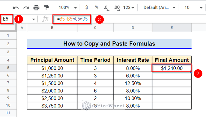
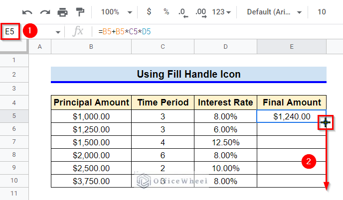
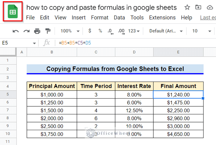
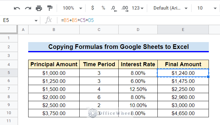
Let’s first get familiar with our datasheet. The datasheet consists of several deposits’ principal amounts, time periods, and interest rates. We have applied simple interest formula to calculate the final amount for the first deposit in Cell E5. Now, we need to copy this formula to other cells of Column E.
1. Apply Paste Special Command
We can apply Copy and Paste Special command from the Edit ribbon to copy formulas to other cells in Google Sheets.
Steps:
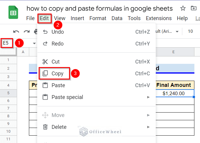
- First, select Cell E5 and then go to the Edit ribbon. Select Copy from the options.
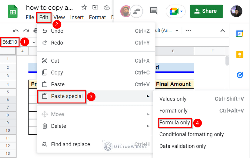
- After that, select the cells where you want to copy the formula (i.e. array E6:E10). Then, go to the Edit ribbon, select the Paste Special option first and Formula Only option later.
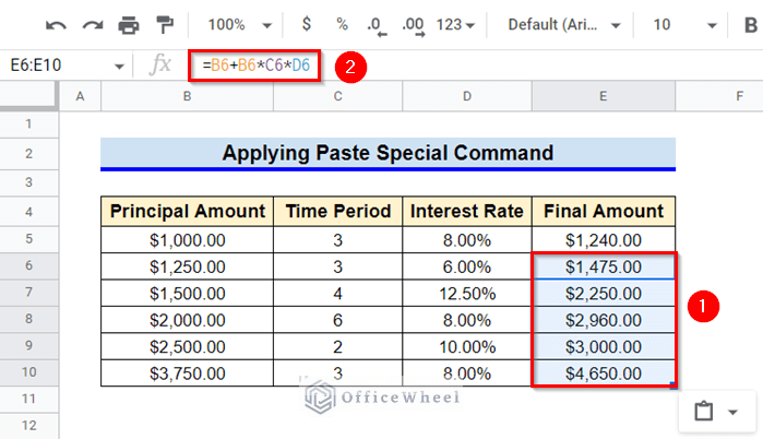
- Now you have values for other cells too. And thus we can copy any formula to other cells.
Read More: How to Copy and Paste in Google Sheets (4 Simple Ways)
2. Use Fill Handle Icon
If the cells where you want to copy any formula are in adjacent rows or columns, then using the Fill Handle icon is the quickest way.
Steps:
- Select Cell E5 and then use the Fill Handle icon to copy the formula by dragging it down.
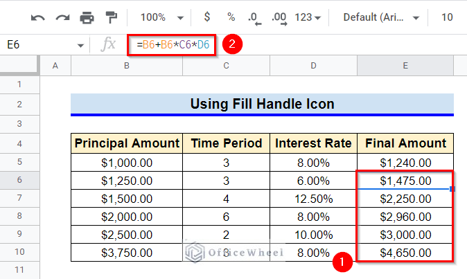
- After dragging down the Fill Handle icon you will have the required values in other cells. An alternative to dragging down the Fill handle is to point the Mouse above it and double-click in left button of the mouse.
Read More: How to Copy and Paste Multiple Rows in Google Sheets (2 Ways)
Similar Readings
- How to Copy and Paste Link in Google Sheets (6 Quick Methods)
- Copy and Paste Multiple Columns in Google Sheets
- How to Copy and Paste Conditional Formatting in Google Sheets
- Copy and Paste Image in Google Sheets (5 Simple Ways)
3. Utilize Keyboard Shortcut
You can also use the Copy and Paste keyboard shortcuts for copying a formula to other cells. Keep reading to learn how.
Steps:
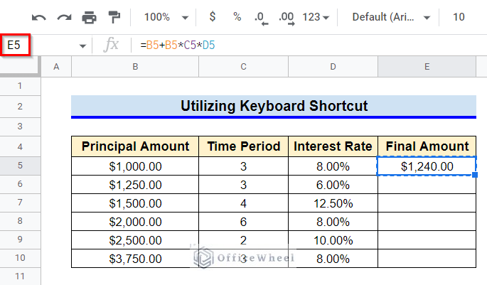
- First, select Cell E5 and use the keyboard shortcut CTRL+C to copy the formula.
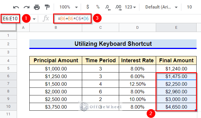
- Now, select array E6:E10 and use the keyboard shortcut CTRL+V to paste the formula and get the required values.
Read More: How to Copy and Paste Multiple Cells in Google Sheets (4 Ways)
4. Apply ARRAYFORMULA Function
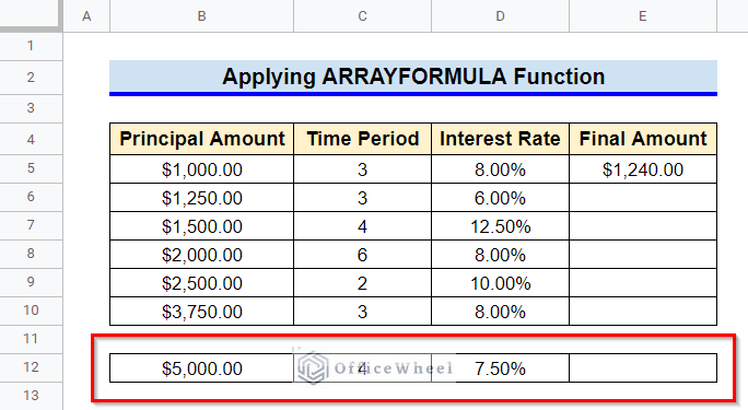
We can use the ARRAYFORMULA function combined with other functions like IF and ISBLANK to apply a formula to an entire column in Google Sheets. To demonstrate the necessity of applying this method, we have made a simple change to our datasheet. We have added a new row after a blank row in the datasheet.
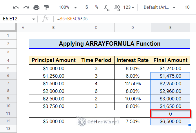
For this simple change, the previously described methods will now not fulfill our requirement. For example, if we apply the Paste Special command, we will get a 0 value for the blank row. But we don’t want any values for a blank row.
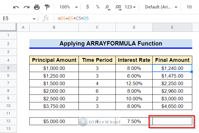
Again, if we use the Fill Handle icon by double-clicking the left button of our mouse, we can’t copy the formula to the newly added row due to the blank row. Therefore, we need to apply the ARRAYFORMULA function.
Steps:
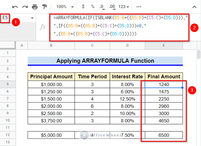
- Delete the current formula in Cell E5 and type in the following formula-
=ARRAYFORMULA(IF(ISBLANK(B5:B+((B5:B)*(C5:C)*(D5:D)))," ",IF((B5:B+((B5:B)*(C5:C)*(D5:D)))=0," ",(B5:B+((B5:B)*(C5:C)*(D5:D))))))- After that, press the Enter key to get the required values ignoring the blank row.
Formula Breakdown
- ISBLANK(B5:B+((B5:B)*(C5:C)*(D5:D)))
First, the ISBLNAK function checks whether any cell in the specified range is empty or not.
- IF(ISBLANK(B5:B+((B5:B)*(C5:C)*(D5:D))),” “,IF((B5:B+((B5:B)*(C5:C)*(D5:D)))=0,” “,(B5:B+((B5:B)*(C5:C)*(D5:D)
Next, the nested IF functions return empty cells if the specified range is empty or has a value of 0.
- ARRAYFORMULA(IF(ISBLANK(B5:B+((B5:B)*(C5:C)*(D5:D))),” “,IF((B5:B+((B5:B)*(C5:C)*(D5:D)))=0,” “,(B5:B+((B5:B)*(C5:C)*(D5:D))))))
Finally, the ARRAYFORMULA function helps with displaying values for the entire column as an array.
How to Copy Formulas from Google Sheets to Excel
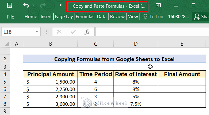
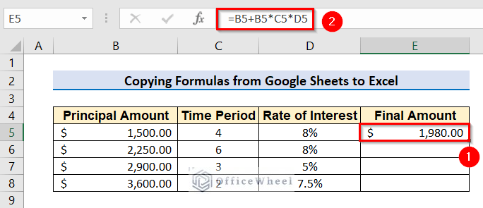
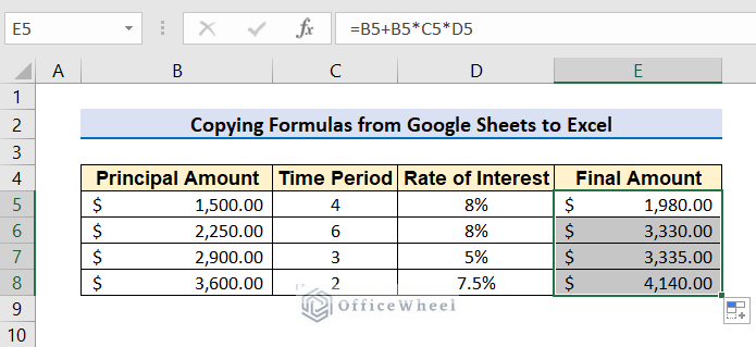
Sometimes we need to work on Google Sheets and MS Excel simultaneously. In such cases, we may need to copy some formulas from Google Sheets to Excel or vice-versa. Here, we have a datasheet in an Excel book which is similar to our datasheet in Google Sheets. Now, go through the following steps to learn how we can copy formulas from Google Sheets to Excel to calculate the required values of the final amount.
Steps:
- First, open your workbook in Google Sheets.
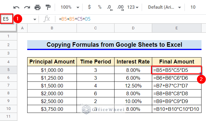
- Now, select Cell E5 and use the keyboard shortcut CTRL+~ to view formulas instead of values.
- Later, again select Cell E5 and use the CTRL+C keyboard shortcut to copy the formula.
- Now, open your Excel workbook.
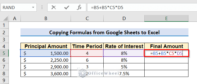
- Activate edit mode in Cell E5 by double-clicking and then Paste the formula by using the CTRL+V keyboard shortcut.
- Press Enter key to get the required value in Cell E5.
- Use any of the methods previously demonstrated to copy the formula in the remaining cells of Column E in the Excel book.
- Return to your Google Sheets workbook and again use the keyboard shortcut CTRL+~ to view values instead of formulas.
Things to Be Considered
- You can copy formulas from one cell only at a time while copying formulas from Google Sheets to Excel.
- The structure of the datasheets in Google Sheets and Excel has to be similar in order to get proper results, otherwise, you will have to modify them after copying.
Conclusion
This concludes our article to learn how to Copy and Paste formulas in Google Sheets. I hope the article was sufficient for your requirements. Feel free to leave your thoughts on the article in the comment box.

