While using Google Sheets, you might occasionally need to convert rows to columns. This doesn’t have to be done manually, one by one. You can accomplish this with ease because of the fantastic capabilities of Google Sheets. In this article, we will show you 3 easy methods to copy horizontal and paste it vertical in Google Sheets.
3 Easy Methods to Copy Horizontal and Paste Vertical in Google Sheets
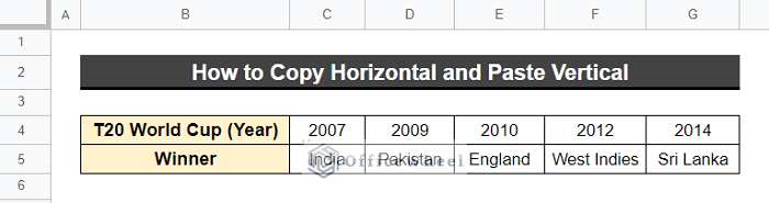
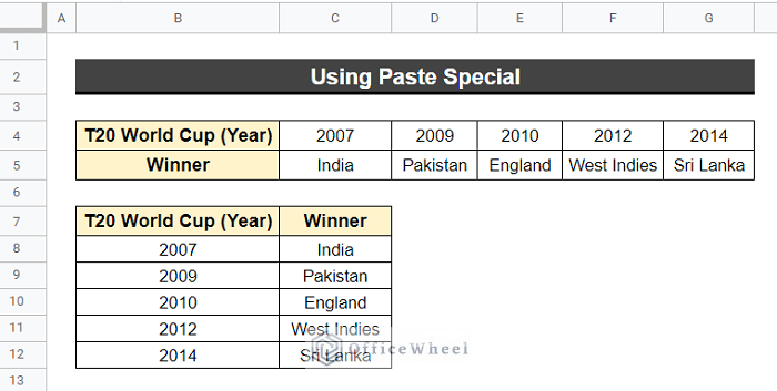
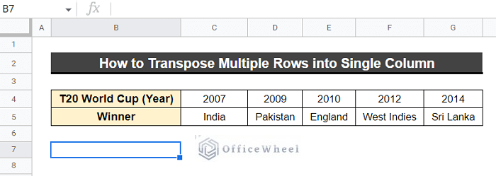
The example of copying data horizontally and pasting it vertically in Google Sheets will be shown using the dataset below. The dataset includes the first five T20 world cup champions. The winner of the T20 World Cup and the year it was held are in two separate rows. In Google Sheets, we wish to paste it along a column.
1. Using Paste Special Command
Using Paste Special command is one the easiest and fastest ways to copy text horizontally and paste it vertically in Google Sheets. The best thing about it is that the format of your data remains the same after transposition.
Steps:
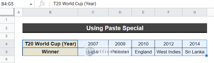
- First, select the entire data range you want to transpose and press the Ctrl+C button.
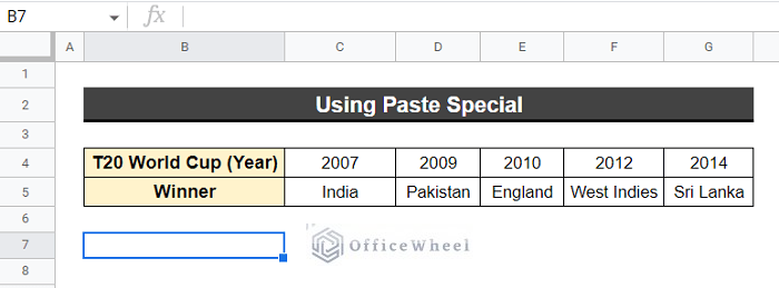
- Now, select a cell in Google Sheets where you want to paste your data.
- Press the right-click button. Go to the Paste special command and select Transposed.
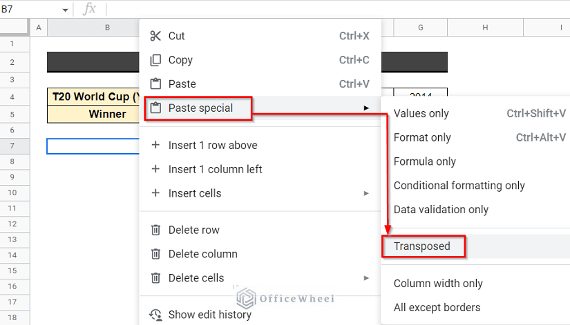
- Google Sheets will paste your data vertically.
Read More: How to Copy and Paste in Google Sheets (4 Simple Ways)
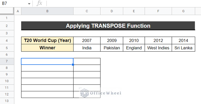
2. Applying the TRANSPOSE Function
We can also use a function in Google Sheets to copy text horizontally and paste it vertically. The TRANSPOSE function will transpose your data but the format of the data changes in this process. The TRANSPOSE function converts the rows and columns in a cell range or an array.
Steps:
- First, select a cell in Google Sheets where you want to paste your data.
- Type the formula below and give your data range inside the TRANSPOSE function–
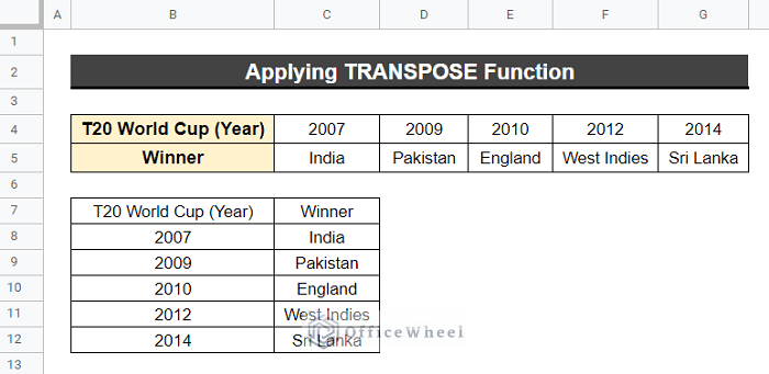
=TRANSPOSE(B4:J5)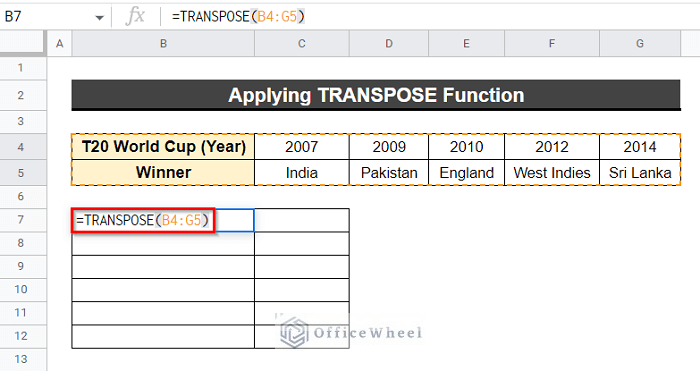
- After pressing the Enter button, you will get your desired result. But it won’t copy the formats.
Read More: How to Copy and Paste Multiple Cells in Google Sheets (4 Ways)
Similar Readings
- How to Copy and Paste Formatting in Google Sheets (5 Ways)
- Copy and Paste Link in Google Sheets (6 Quick Methods)
- How to Copy and Paste Conditional Formatting in Google Sheets
- Copy and Paste Image in Google Sheets (5 Simple Ways)
3. Employing INDEX Function to Transpose Every N Rows into Columns
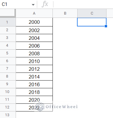
We can copy horizontally and paste vertically in a slightly different way. Like, you may want to copy every n number of rows of a column and paste n number of columns at a time; you can use the INDEX function to do so. The INDEX function gives back the cell’s content which is specified by the row and column offset. But for this method, It will need to start the dataset from Cell A1, otherwise, the formula won’t work properly.
Steps:
- Choose a cell where you want to paste your data. We chose Cell C1.
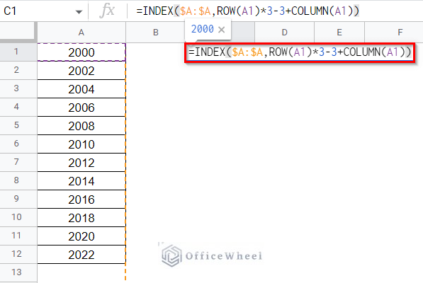
- Now, type the function below and press Enter–
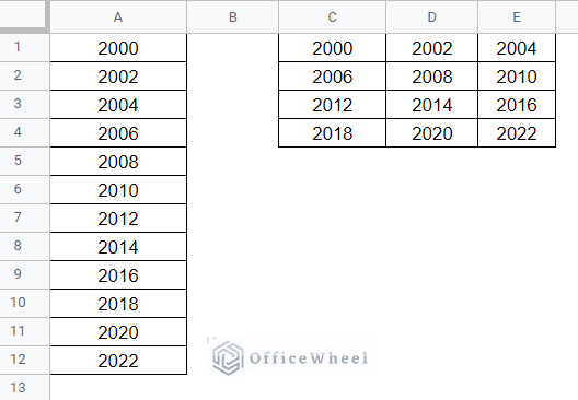
=INDEX($A:$A,ROW(A1)*3-3+COLUMN(A1))where N represents how many rows you wish to transpose at once. We want to transpose every 3 rows of Column A to 3 columns, so we use (N = 3).
Formula Breakdown
- ROW(A1)
It indicates the row where Cell A1 is located.
- COLUMN(A1)
It designates the column that contains Cell A1.
- INDEX($A:$A,ROW(A1)*3-3+COLUMN(A1))
Here, $A:$A specifies the set of cells where the values are extracted. ROW(A1)*3-3+COLUMN(A1) indicates the values to be returned from the set of cells.
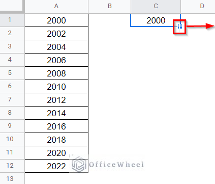
- Now, drag the Fill Handle icon towards the right direction up to 3 columns.
- Then drag the Fill Handle icon towards the down direction.
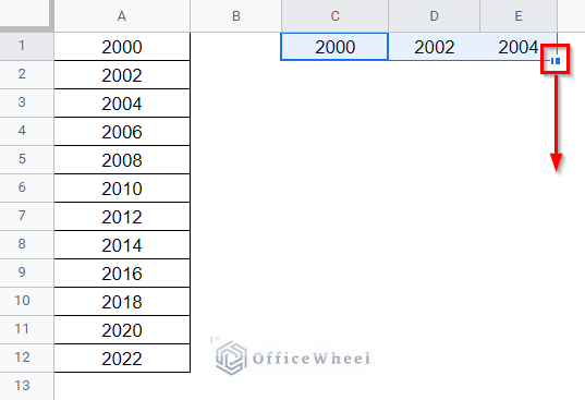
- Now see, it created three columns which are showing every third row from the column.
Read More: How to Copy and Paste Multiple Rows in Google Sheets (2 Ways)
How to Transpose Multiple Rows into a Single Column
Sometimes, you may wish to transpose multiple rows into a single column in Google Sheets. You can use the FLATTEN function to do so. All the values from one or more ranges are squashed into a single column by the FLATTEN function.
Steps:
- First, select a cell in Google Sheets where you want to paste your data.
- Now, type the function below and press the Enter button-
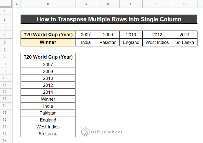
=FLATTEN(B4:G5)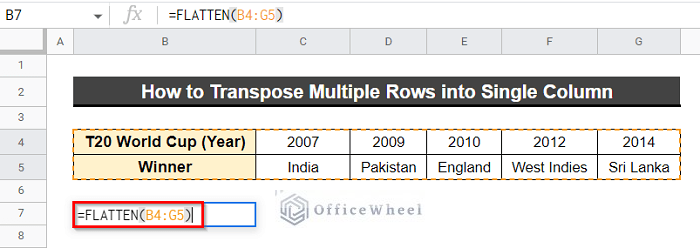
- Soon after, we’ll get all the data in a single column.
Read More: How to Copy and Paste Multiple Columns in Google Sheets
Conclusion
In Google Sheets, you may wish to copy text horizontally and paste it vertically. In this article, we have demonstrated how to do so by using the Paste Special command, the TRANSPOSE function. We have used the INDEX function to transpose every N row into N columns, and we have used the FLATTEN function to transpose multiple rows into a single column.
In the comments box below, feel free to ask any questions or suggest any ideas. For additional information, please visit Officewheel.com.