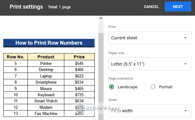
Sometimes we need to print the row numbers of our dataset in Google Sheets. But you can’t print the row numbers by default because rows and columns are out of the print area in Google Sheets. For getting the row numbers you can use the built-in function i.e. ROW function or apply some other methods. In this article, I’ll show you 4 useful methods about how to print row numbers in Google Sheets with clear images and steps. After the methods, you’ll get an output like the below picture having the row numbers beside your dataset.
A Sample of Practice Spreadsheet
You can download Google Sheets from here and practice very quickly.
4 Useful Methods to Print Row Numbers in Google Sheets
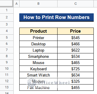
Let’s get introduced to our dataset first. Here we have some products in Column B and their prices in Column C. We are seeing the row numbers beside our dataset. If we want to print our dataset by default method, then the row numbers won’t print at all. So, we’ll see 4 useful methods about how to print row numbers in Google Sheets by using this dataset below.
1. Applying Fill Handle Tool
First and foremost, we’ll apply the Fill Handle tool to print row numbers in Google Sheets. This process is a bit lengthy because first, we have to insert the first 2 row numbers manually. Then we can use the Fill Handle tool to get the rest of the row numbers in a moment. Let’s see the process.
Steps:
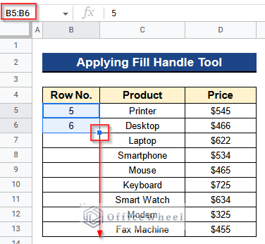
- Firstly, type 5 in Cell B5 because it is in Row 5.
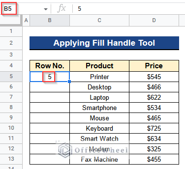
- Moreover, write 6 in Cell B6.
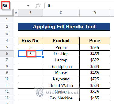
- Secondly, select Cells B5 and B6 and apply the Fill Handle tool in the rest of the cells of Column B. It will automatically detect the pattern and fill in the row numbers.
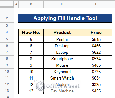
- Then, you’ll see the row numbers in Column B.
- Now we’ll print this dataset with the row numbers.
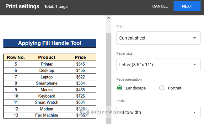
- Finally, press Ctrl+P on your keyboard to go to the Print Settings window. You’ll find that your dataset now has the row numbers beside the products and prices. You can easily print your dataset now from this window.
Read More: How to Print Header on Each Page in Google Sheets
2. Using ROW Function
Apart from the previous method, we can use the ROW function to obtain the row numbers quickly. This function gives the row number of the given cell very fast. Then we can print the output easily having the row numbers beside our values in the dataset. Let’s see how to do it.
Steps:
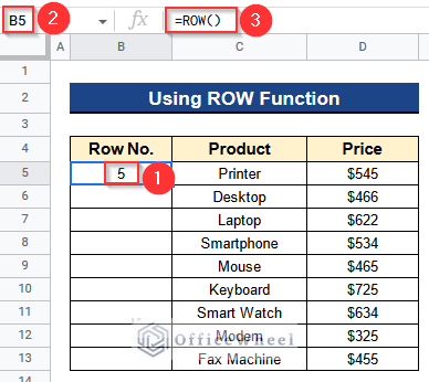
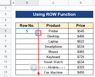
- At first, write the following formula in Cell B5–
=ROW()- Then, press Enter to get the corresponding row number.
- Next, use the Fill Handle tool to apply the formula to the rest of the cells of Column B.
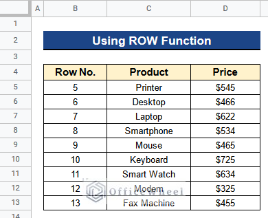
- Then, the row numbers will be in Column B.
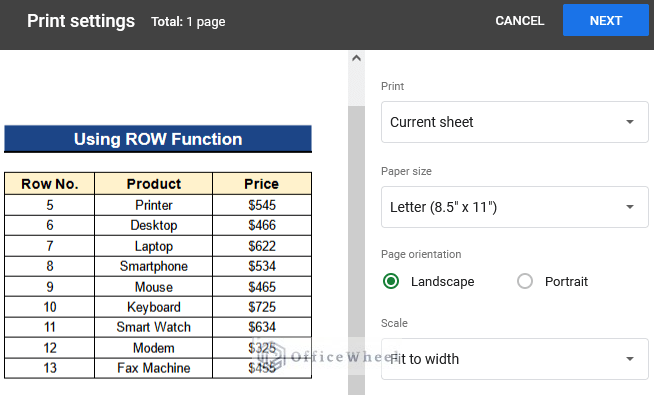
- At last, press Ctrl+P from your keyboard to open the Print Settings window.
- Then, you can easily print your dataset having the row numbers.
Read More: How to Print Only Certain Columns in Google Sheets (3 Ways)
Similar Readings
- How to Print Bigger in Google Sheets (2 Simple Examples)
- Print Preview in Google Sheets (2 Easy Examples)
- How to Print Mailing Labels from Google Sheets (With Easy Steps)
- Print to PDF Using Apps Script in Google Sheets
3. Merging IF and ROW Functions
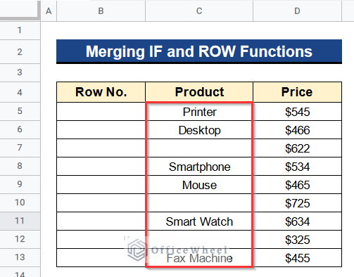
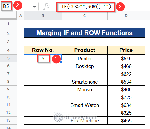
Now we have a slightly different dataset as you can see in the picture. Some products are missing in Column C. In addition, we only need the row numbers for the current values, not for all the values. We can do that by merging the IF and ROW functions together. The IF function searches for any given logic within our dataset and produces results instantly. Here it will search for non-empty cell in Column C of our dataset and gives only their row numbers with the help of the ROW function.
Steps:
- First of all, select Cell B5 and insert the formula there-
=IF(C5<>"",ROW(),"")- Next, to obtain the corresponding row number, hit Enter.
Formula Breakdown
- ROW()
Firstly, this function gives the row number of the given cell, which is Cell C5.
- IF(C5<>””,ROW(),””)
Then, this function searches whether Cell C5 is empty or not. If the logical expression is TRUE, it will give nothing. But when the logical expression is FALSE then it will return the corresponding row number.
- After that, apply the formula to the remaining cells in Column B using the Fill Handle tool.
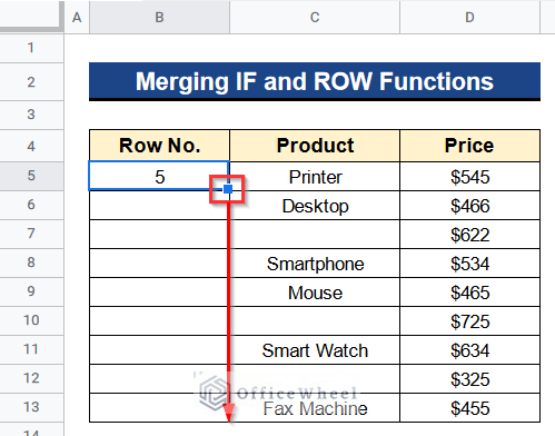
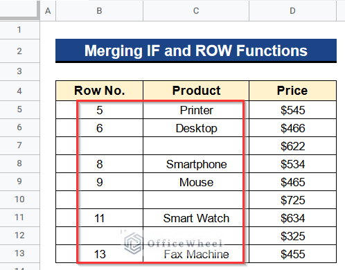
- Consequently, Column B will contain the row numbers for those cells of Column C that are not empty.
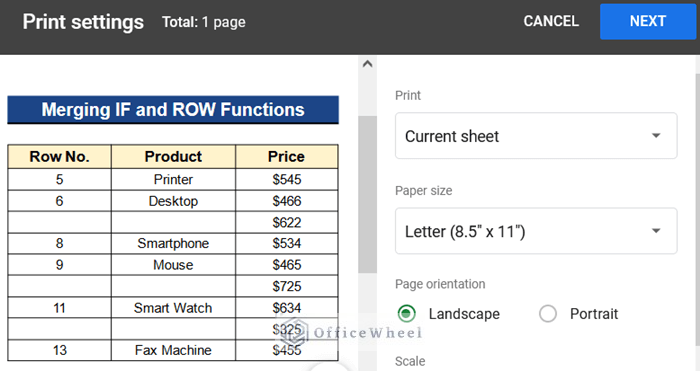
- Ultimately, using your keyboard, press Ctrl+P together to bring up the Print Settings window.
- After that, printing your dataset with the row numbers is so simple.
Read More: How to Print in Landscape in Google Sheets (2 Simple Ways)
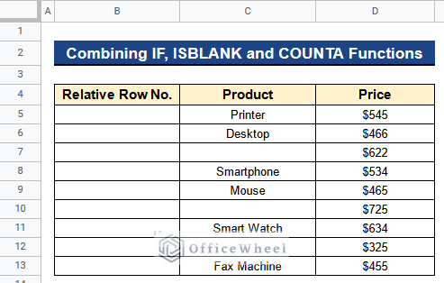
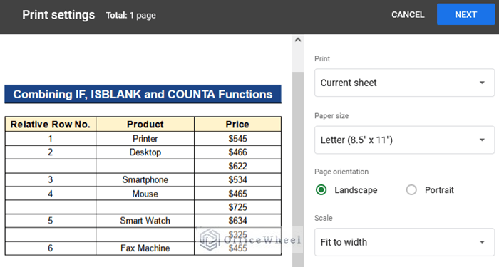
4. Combining IF, ISBLANK and COUNTA Functions
Apart from the previous method now we don’t want the actual row numbers. We want the relative row numbers of our products that are present in Column C. In order to do that, I’ll combine the IF, ISBLANK, and COUNTA functions to get the relative row numbers of our products. Below you’ll find the process.
Steps:
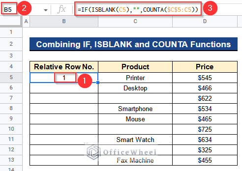
- Before all, activate Cell B5.
- Then, type the below formula in it-
=IF(ISBLANK(C5),"",COUNTA($C$5:C5))- Next, press Enter to get the relative row number with respect to the values present in the dataset.
Formula Breakdown
- COUNTA($C$5:C5)
Firstly, this function counts the number of values from Cells C5 to C5.
- ISBLANK(C5)
Then, this function checks if Cell C5 is empty or not.
- IF(ISBLANK(C5),””,COUNTA($C$5:C5))
Finally, this function checks whether Cell C5 is empty or not with the help of the ISBLANK function. The logical expression will produce nothing if it is TRUE. But when the logical expression is FALSE then it will return the relative row number with the help of the COUNTA function.
- Again, utilizing the Fill Handle tool, apply the formula to the remaining cells in Column B.
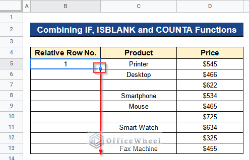
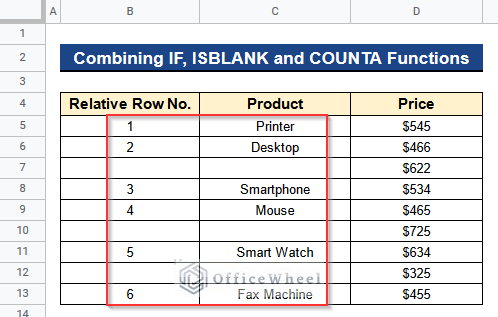
- Then, you’ll see the relative row numbers in Column B.
- You’ll get the relative row numbers for only those values of Column C which are present in the dataset. We won’t get the relative row numbers for the empty cells.
- In the end, use your keyboard’s Ctrl+P shortcut to open the Print Settings window.
- Your dataset will now include the relative row numbers next to the available products and prices. Now that you have this window, you may quickly print your dataset.
Read More: How to Print Google Sheets on One Page (2 Distinct Scenarios)
Conclusion
That’s all for now. Thank you for reading this article. In this article, I have discussed 4 useful methods about how to print row numbers in Google Sheets. Please comment in the comment section if you have any queries about this article. You will also find different articles related to google sheets on our officewheel.com. Visit the site and explore more.