Use REGEXREPLACE to Replace Multiple Values in Google Sheets (An Easy Guide)

While there are a number of ways to do so, the REGEXREPLACE function is a great way to replace multiple values in Google Sheets, especially for string conditions.

The function can take advantage of regular expressions to customize string conditions exactly to the users’ needs.

Table of Contents

How to Use REGEXREPLACE to Find and Replace a Value

Note: This section covers the fundamentals of the REGEXREPLACE function. You can skip ahead to the next section for the main methods. However, we recommend you read through this section as well.

Primarily, it is the SUBSTITUTE function that comes to mind when we think about replacing values in Google Sheets. However, the REGEXREPLACE function takes things further by allowing regular expressions to be used to further customize the search results.

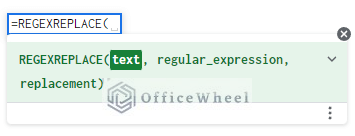
The REGEXREPLACE function syntax:

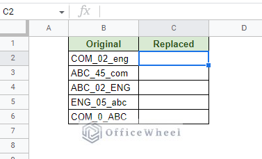
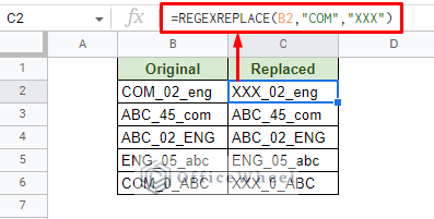
REGEXREPLACE(text, regular_expression, replacement)

Let’s use the following dataset to show how we can use the REGEXREPLACE function to replace a value in Google Sheets.

Here, let’s replace the string “COM” with “XXX”:

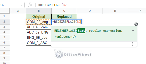
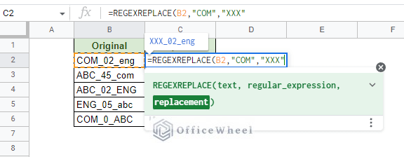
Step 1: Open the function and input the cell reference of the source value. In this case, it is cell B2.

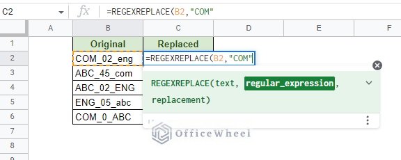
Step 2: The next field is for the regular expression, but in this case, we will input the text we want to replace, “COM”. The regular expression must be inside quotation marks (“”).

Step 3: Input the replacement string next. For this example, it is “XXX”.

You can see a preview of the result of the formula.

Step 4: Close parentheses and press ENTER to apply. Then use the fill handle to apply the formula to the rest of the column.

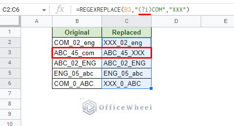
=REGEXREPLACE(B2,"COM","XXX")

Notice that the formula is case-sensitive. But worry not, there is a way to make it case-insensitive.

Making REGEXREPLACE Case-Insensitive with Regular Expression

We can easily make the REGEXREPLACE function case-insensitive by using the following regular expression flag:

(?i)

Simply place it in from of the searched string in the regular expression field:

=REGEXREPLACE(B2,"(?i)COM","XXX")

With the fundamentals out of the way, let’s now see how we can use the REGEXREPLACE function to replace multiple values in Google Sheets.

Similar Readings

How to Use REGEXREPLACE to Replace Multiple Values in Google Sheets

1. Using OR Condition to Replace Multiple Values with the Same Result in Google Sheets

While the REGEXREPLACE function can be used like the SUBSTITUTE function to replace multiple values, the function has the advantage of being able to use regular expression conditions to operate.

The condition in question is the OR condition, represented by the vertical bar (|).

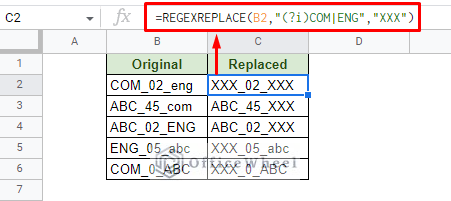
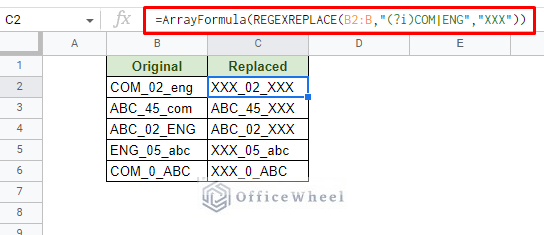
Here’s a simple example: Replace both “COM” or “ENG” strings with “XXX”, regardless of the case.

With SUBSTITUTE, we’d have to nest the function for each condition:

=SUBSTITUTE(SUBSTITUTE(B2,"COM","XXX"),"ENG","XXX")

And two more nests for the lower-case results.

On the other hand, with REGEXREPLACE the formula is simply:

=REGEXREPLACE(B2,"(?i)COM|ENG","XXX")

This is also case-in-sensitive, thanks to the (?i) regular expression flag.

However, it is crucial to understand that using the vertical bar (|) condition is only viable if we are replacing multiple values with the same result, which in this case was “XXX”.

Use the ARRAYFORMULA Function to Instantly Cover a Large Range of Data

Using the ARRAYFORMULA function around our formula gives us three advantages:

We get to input a range of values, making the formula dynamic and accepting new entries.
It allows the user to input the formula only once, saving the need to use the fill handle down the column.
This also reduces the processing time that the application needs.

That said, the first change we need to bring to the formula is to update the data range from B2 to B2:B.

The second is to apply the ARRAYFORMULA function itself around the formula. You can do this easily by putting the text cursor at the end of the formula and pressing CTRL+SHIFT+ENTER on your keyboard. Manual input of the function is also possible.

The formula should look like this:

=ArrayFormula(REGEXREPLACE(B2:B,"(?i)COM|ENG","XXX"))

2. Using Nested REGEXREPLACE Functions to Replace Multiple Values in Google Sheets

If you have multiple values to replace with other different values, you must resort to the nested function method.

Here, for each different result, we will have one more nested REGEXREPLACE function.

For example, in our existing formula, we want to add another condition. That is to replace the underscores (_) with dashes/hyphens (-).

The formula is:

=ArrayFormula(REGEXREPLACE(REGEXREPLACE(B2:B,"(?i)COM|ENG","XXX"),"_","-"))

The more conditions you add, the more REGEXREPLACE functions must be included in the nest.

Final Words

The use of the REGEXREPLACE function to replace multiple values in Google Sheets is quite similar to SUBSTITUTE, however, it has some advantages over it mostly in the form of the use of regular expressions.

Regular expressions are a great approach when it comes to customizing searches for strings.

Feel free to leave any queries or advice you might have for us in the comments section below.