We often need to remove duplicate entries from our spreadsheet. When you have a huge dataset, you may get repetition of multiple data but then you just need to know the unique data only. That’s why filtering unique values is important. In this article, we have demonstrated 4 easy methods on how to filter unique rows in Google Sheets.
A Sample of Practice Spreadsheet
Here is the spreadsheet used for explaining the methods. You can easily download it from here.
4 Easy Methods to Filter Unique Rows in Google Sheets
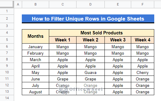
There are several ways to filter unique values from multiple rows. Here, the 4 easiest methods are described. We will be using the following dataset for an example. The dataset represents the most sold products of a grocery shop in the first 8 months.
1. Using UNIQUE Function
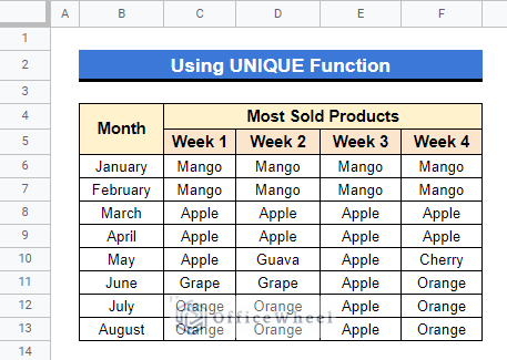
The UNIQUE function eliminates duplicate rows from the source range and returns only unique records. Assume, in the following dataset, we want to remove the duplicate rows and get the unique rows only.
Steps:
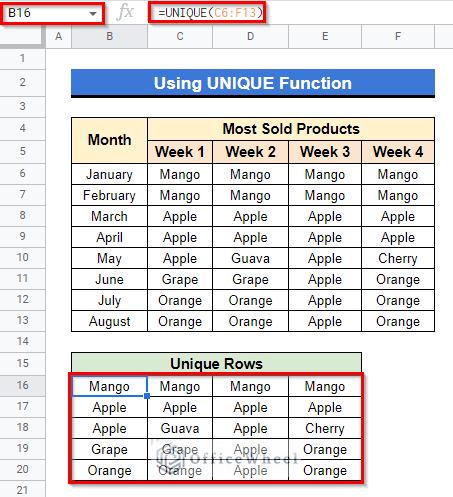
- First, select Cell B16 in the following dataset, then apply the below formula and press Enter–
=UNIQUE(C6:F13)The formula simply looks for the unique rows from the Cell range C6:F13 and returns them.
Read More: How to Remove Unique Values in Google Sheets (2 Suitable Ways)
2. Combining ARRAYFORMULA with UNIQUE Functions
We use the ARRAYFORMULA function to ignore the repetition of continuous formula entering. Here, we’ll join it with the UNIQUE function.
Steps:
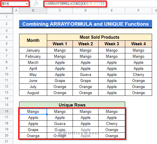
- Pick out Cell B16 in the consequent spreadsheet, then attach the following formula on that cell and press Enter–
=ARRAYFORMULA(UNIQUE(C6:F13))Formula Breakdown
- UNIQUE(C6:F13)
Filter unique rows only.
- ARRAYFORMULA(UNIQUE(C6:F13))
Avoid repetition of filtering unique rows procedure for further inputs and return output as an array.
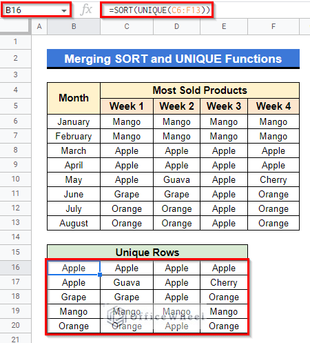
3. Merging SORT and UNIQUE Functions
Do you want to filter unique rows and get them in alphabetical order? The SORT function in Google Sheets is built for that. Combining it with the UNIQUE function will return the sorted unique rows.
Steps:
- At first, select Cell B16 in the following dataset, apply the formula given below, press Enter and there you go!
=SORT(UNIQUE(C6:F13))Formula Breakdown
- UNIQUE(C6:F13)
Filter out just distinct rows.
- SORT(UNIQUE(C6:F13))
Arrange the filtered rows in alphabetical order.
4. Applying Custom Formula in Filter Menu
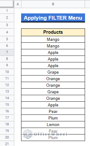
You can use a custom formula option from the filter menu and then apply a specific formula to filter unique values as well. Suppose, in the following dataset, we want to filter unique values from the single column using the filter menu.
Steps:
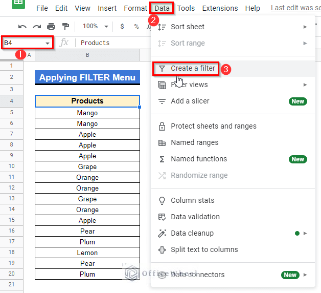
- At first, choose Cell B4, then at the toolbar, go to the Data option and select Create a filter.
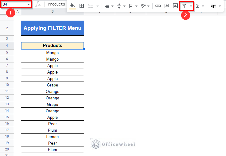
- Or, you can simply click on the Create a filter ribbon at the toolbar.
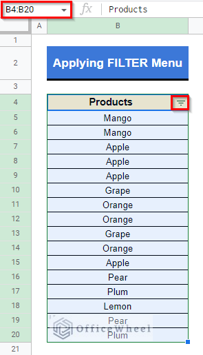
- After that, the filter option will be created for the Cell range B4:B20.
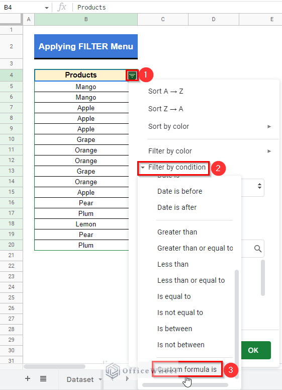
- Now, at the right of Cell B4, select the dashed Filter Ribbon, then select Filter by condition, and after that choose Custom formula is
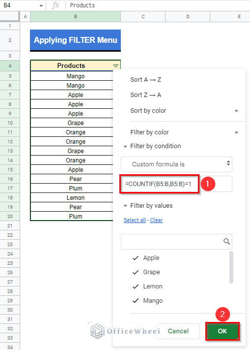
- Apply the following formula in the “Value or formula” bar then select OK.
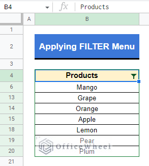
=COUNTIF(B5:B,B5:B)=1- And you will get the output as you wanted.
Read More: Use COUNTIF Function to Count Unique Values in Google Sheets
How to Filter Unique Rows Ignoring Blank Cells in Google Sheets
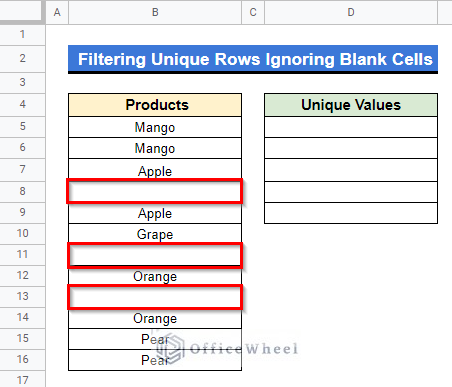
There can stay one or more blank cells in a huge spreadsheet and while filtering unique values, you may not want to count them as a unique value. There is a solution for that as well. Using the combination of UNIQUE and FILTER functions easily solves the matter. Presume, in the following dataset, you want to ignore those blank cells while filtering unique values.
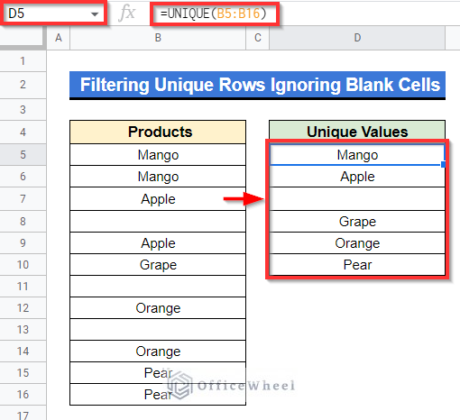
Now, if we apply only the following UNIQUE formula in Cell D5 here, what will happen?
=UNIQUE(B5:B16)We can see that the UNIQUE function is counting those blank cells and showing a unique blank cell as output. Obviously, we have a solution for that. If we use the FILTER function along with the UNIQUE function, the FILTER function will filter all values except those blank cells first.
Steps:
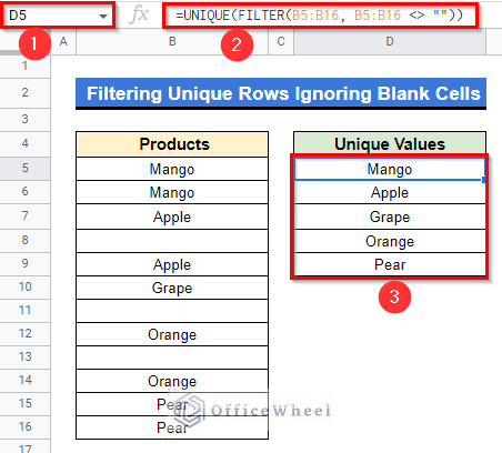
- First, activate Cell D5, embed there the following formula below, and press Enter–
=UNIQUE(FILTER(B5:B16, B5:B16 <> ""))Now see, no blank rows are remaining in the filtered range.
Formula Breakdown
- FILTER(B5:B16, B5:B16 <> “”)
Filter all values except blank cells.
- UNIQUE(FILTER(B5:B16, B5:B16 <> “”))
Filter unique values from the previously filtered values.
Read More: How to Get Unique Values Without Blanks in Google Sheets
Conclusion
From a large dataset, where there is repeated data, filtering unique values only is an important task often. The article elucidated 4 easy methods to filter unique rows in Google Sheets. Hope this helps with your work. Visit our site officewheel.com to see more related articles. Thank you.

