How to Highlight Unique Values in Google Sheets (9 Useful Ways)

Conditional Formatting is a dynamic tool for performing several operations swiftly in Google Sheets. We can apply several conditions to our dataset by using this tool. We can also insert several functions like the UNIQUE function into the Conditional Formatting tool in order to highlight the distinct values only. In this article, we’ll see 9 useful ways to highlight unique values in Google Sheets with clear steps and images.

A Sample of Practice Spreadsheet

You can download Google Sheets from here and practice very quickly.

9 Useful Ways to Highlight Unique Values in Google Sheets

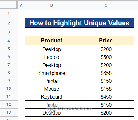
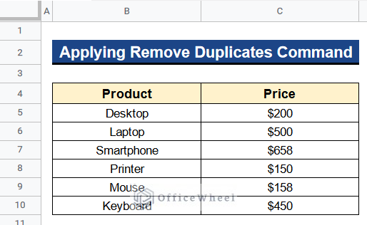
Let’s get introduced to our dataset first. Here we have some products in Column B and their prices in Column C. There are some unique values and some duplicate values in both Columns B and C. We want to highlight the unique values only. So, I’ll show you 9 useful ways to highlight unique values in Google Sheets by using this dataset.

1. Using UNIQUE Function

First and foremost, we can use the UNIQUE function to obtain the unique values out of duplicates in Google Sheets. This function simply brings out the distinct values from duplicate values very fast. Let’s see the steps.

Steps:

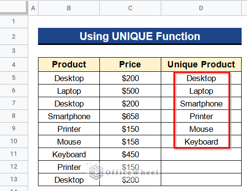
• Firstly, type the following formula in Cell D5–

• Secondly, hit Enter to get the unique products list.

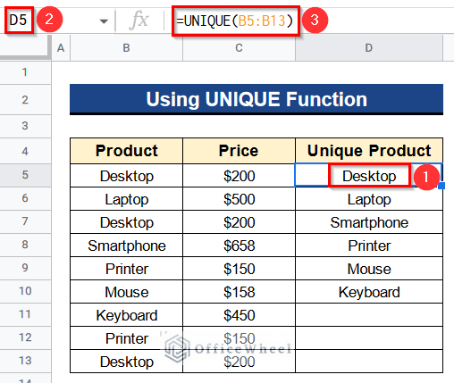
• Finally, you’ll get the names of the unique products in Column D.

Read More: How to Use Pivot Table to Count Unique Values in Google Sheets

2. Assigning SORT Function

Now we will assign another function which is the SORT function. This function sort any textual values alphabetically. This process doesn’t directly give unique values. But if we use this function, we’ll find the sorted values quickly. Then from the sorted values, we can identify the duplicates. After that, we can remove them manually. Here are the procedures.

Steps:

• At first, select Cell D5.
• Then, insert the following formula there-

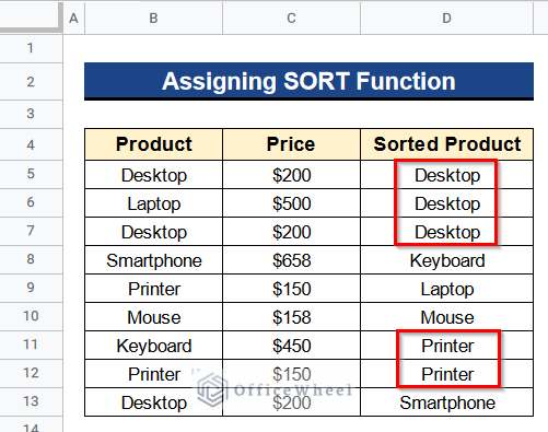
• Next, press Enter to get the sorted products list.

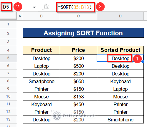
• At last, you’ll find all the products sorted alphabetically in Column D. Now, you can easily find out the duplicates and can remove them manually.

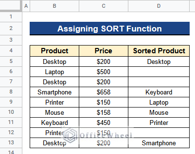
• Finally, we removed the duplicate values manually by pressing the Delete key from the keyboard and got the unique products in Column D.

3. Applying Remove Duplicates Command

Another quickest method to remove duplicates and obtain the unique values is to use the Remove Duplicates command. This command directly removes any duplicates within any given range in the dataset and produces the result. Below we’ll see the procedures.

Steps:

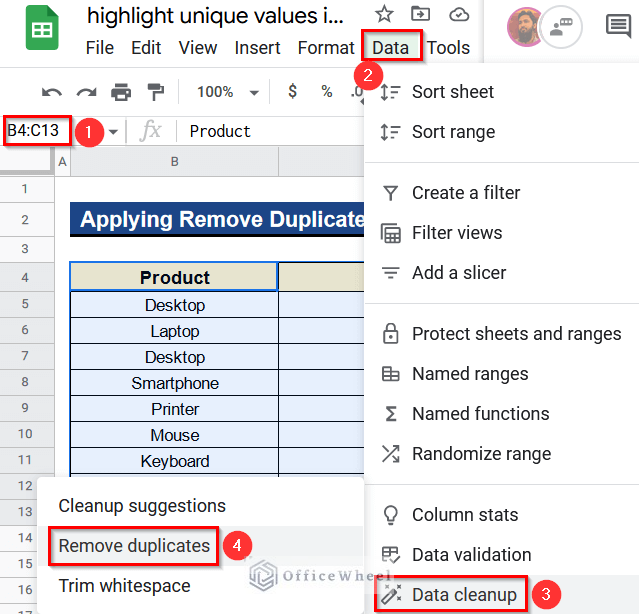
• First of all, select all the cells from Cell B4 to C13.
• After that, go to Data > Data Cleanup > Remove Duplicates.

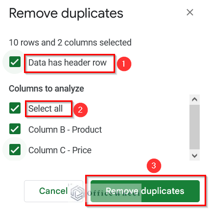
• Remove Duplicates window will open.
• Select Data has header row and Select all options under this window.
• Then, click on the Remove Duplicates button.

• After that, you’ll get a message like below that the duplicates are removed.

• In the end, there will be only the unique values of both products and prices in the dataset.

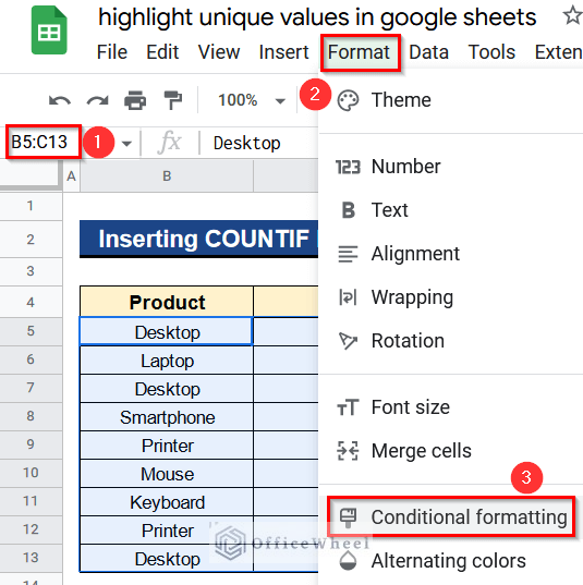
4. Inserting COUNTIF Function

Apart from the previous method, we can use the Conditional Formatting tool to highlight unique values in Google Sheets. For this, we have to insert the COUNTIF function into the Conditional Formatting tool. The COUNTIF function will count the unique values in our dataset and will highlight them with our given color. You’ll find the process below.

Steps:

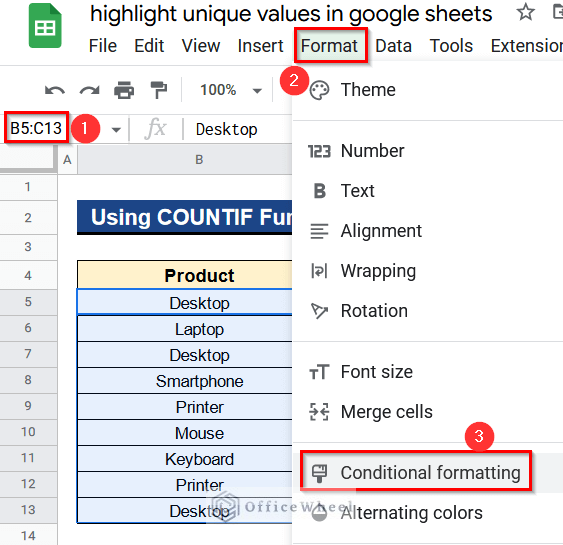
• First, select every cell from Cell B5 through Cell C13.
• Thereafter, go to Format > Conditional Formatting.

• Afterward, the Conditional Format Rules window will open.
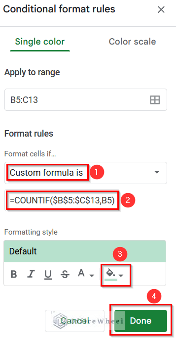
• Consequently, select Custom Formula Is under the Format Rules menu.
• Then, put the following formula into the formula box-

• Next, select the green color from the color box.
• After that, click on the Done button.

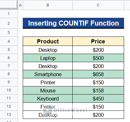
• Ultimately, we highlight the unique values in green color both in Columns B and C.

Read More: Use COUNTIF Function to Count Unique Values in Google Sheets

5. Combining ARRAYFORMULA and COUNTIF Functions

We can also combine the ARRAYFORMULA and COUNTIF functions into the Conditional Formatting tool to highlight the unique values. The advantage of this method is that we can extend the range of our calculation. The ARRAYFORMULA expands the results along the whole dataset promptly.

Steps:

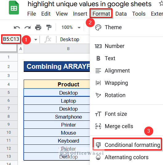
• In the first place, choose all of the cells from Cell B5 to Cell C13.
• After that, select Conditional Formatting under the Format menu.

• The Conditional Format Rules window will then appear.
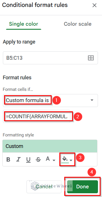
• Next, choose Custom Formula Is from the Format Rules menu.
• Then, put the formula listed below into the formula box-

• Choose green from the color box next.
• Click the Done button after that.

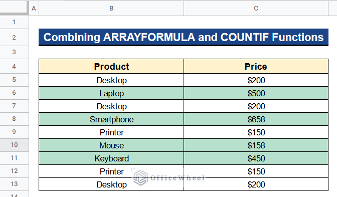
• Finally, we mark the distinctive values in both Columns B and C using the color green.

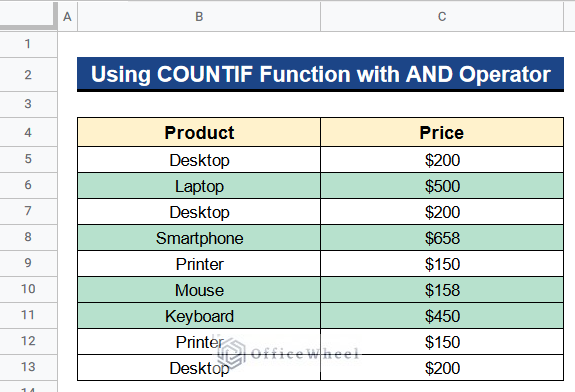
6. Using COUNTIF Function with AND Operator

Besides the former method, we can use the COUNTIF function with the AND operator (*) to extend our calculation in order to highlight unique values in Google Sheets. We can add several COUNTIF functions together with the AND operator (*) into the Conditional Formatting tool to increase the range of our results. Now check out the procedures below.

Steps:

• Before all, select every cell from Cell B5 through Cell C13.
• Go to Format > Conditional Formatting then.

• After that, a window called Conditional Format Rules will appear.
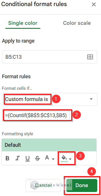
• As a result, choose Custom Formula Is from the Format Rules menu.
• Further, add the following formula to the formula box-

• Next, choose the color green from the color box.
• Click the Done button once you’re finished.

• In the end, we use the color green to highlight the unique values in both Columns B and C.

7. Merging MATCH and UNIQUE Functions

Now we want to highlight only one column of our dataset. That is Column B, the products column. So we can do this by merging the MATCH and UNIQUE functions into the Conditional Formatting tool. The UNIQUE function finds out the unique values and the MATCH function gives their relative position in order to highlight them.

Steps:

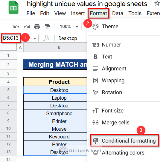
• Earlier on, select all the cells from Cell B5 to C13.
• Consequently, continue by selecting Format > Conditional Formatting.

• A screen called Conditional Format Rules will then appear.
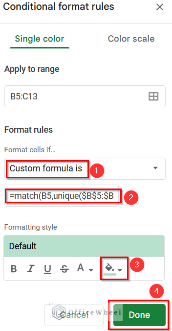
• In light of this, choose Custom Formula Is from the Format Rules menu.
• In the formula box, type the following formula-

• Then, tap the color box and choose green.
• Select the Done button following that.

• Ultimately, we only highlight the unique values of Column B in green color which is the products list.

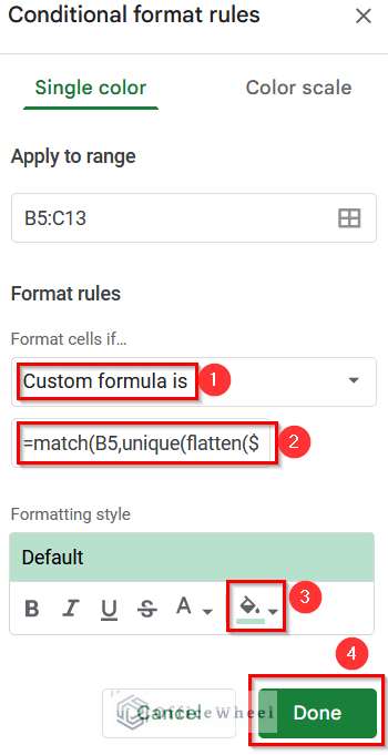
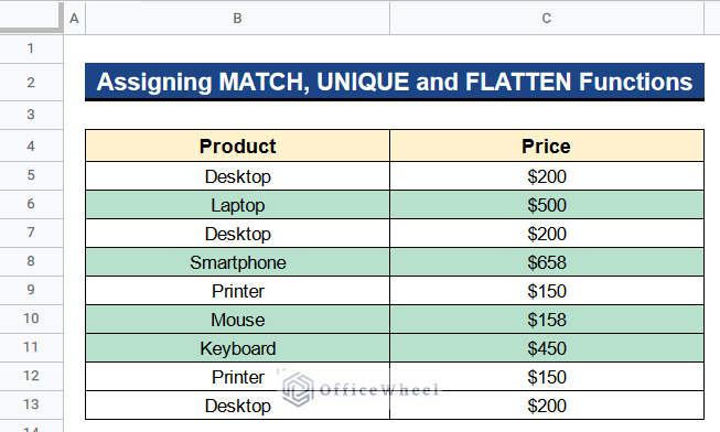
8. Assigning MATCH, UNIQUE and FLATTEN Functions

The previous method only gives results for just one column, Column B. But now if we want to increase our result into another column, Column C we can do it by assigning the MATCH, UNIQUE, and FLATTEN functions together. Here, the FLATTEN function makes the 2 columns, Columns B and C a single column, and then with the help of the UNIQUE, and FLATTEN functions, we get the unique values highlighted.

Steps:

• Initially, the cells from Cell B5 to Cell C13 should all be selected.
• Then, select Format > Conditional Formatting.

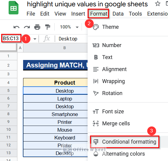
• Next, the Conditional Format Rules window will appear.
• Consequently, choose Custom Formula Is from the Format Rules menu.
• Then, enter the following formula into the formula box-

• Next, pick the color green from the color box.
• After that, press the Done Button.

• Finally, both Columns B and C‘s distinctive values are highlighted in green.

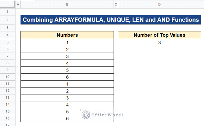
9. Combining ARRAYFORMULA, UNIQUE, LEN and AND Functions

Let’s look into another problem. Suppose we have a dataset of numerical entries where we want to highlight the top n values of the dataset. We can do this by combining the ARRAYFORMULA, UNIQUE, LARGE, N, LEN, and AND functions into the Conditional Formatting tool. These functions enable us to highlight our desired result. We can have our values in a column or in a row. We’ll see both procedures below.

9.1 Highlighting Top N Values in Column

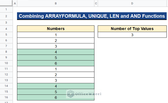
We have a dataset where we have the numerical entries in Column B. And we want to highlight the top 3 values of our dataset. Let’s see the process.

Steps:

• First and foremost, select all the cells from Cell B5 to B16.
• Moreover, pick Conditional Formatting under the Format menu.

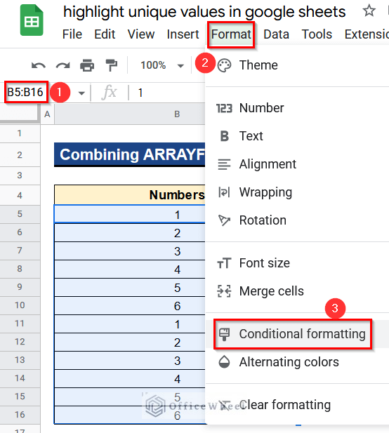
• Afterward, you’ll see a window called the Conditional Format Rules.
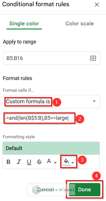
• Apart from this, select Custom Formula Is under the Format Rules menu.
• Next, into the formula box type the below formula-

• Then, green color should be chosen.
• Lastly, press the Done

• Finally, we highlight the top 3 values of Column B in green color which are 4, 5, and 6.

9.2 Highlighting Top N Values in Row

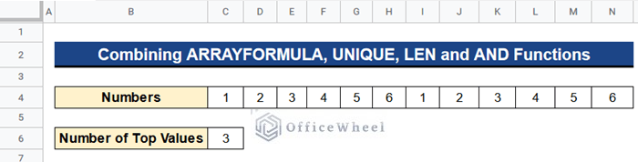
Now, we have our values in Row 4. Here we also want to highlight the top 3 values of our dataset.

Steps:

• Firstly, choose every cell from Cell C4 through Cell N4.
• Again, go to Format > Conditional Formatting.

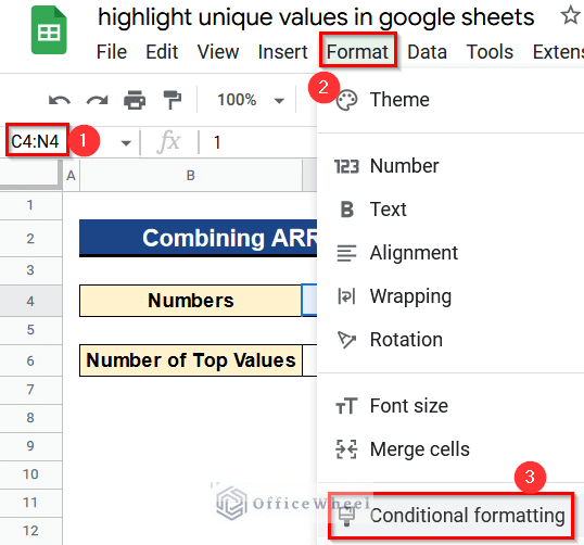
• Moreover, you will move to the Conditional Format Rules window.
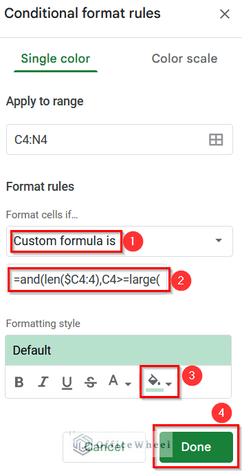
• From this window, pick Custom Formula Is below the Format Rules menu.
• After that, type the next formula-

• Next, pick the green color from the color box.
• After that, click on the Done button to finish the task.

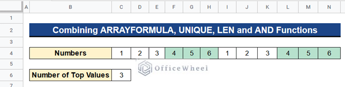
• In the end, we highlight in green the top 3 values of Row 4, which are 4, 5, and 6.

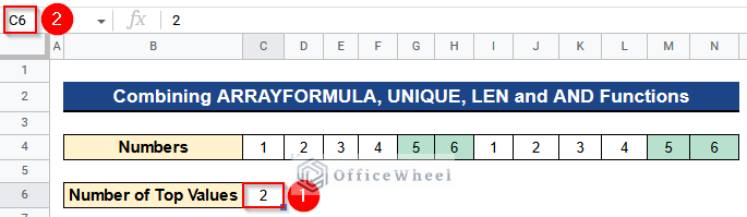
• We change the number of top values from 3 to 2 in Cell C6 and you can see that now it is highlighting the top 2 values in Row 4.

Conclusion

That’s all for now. Thank you for reading this article. In this article, I have discussed 9 useful ways to highlight unique values in Google Sheets. Please comment in the comment section if you have any queries about this article. You will also find different articles related to google sheets on our officewheel.com. Visit the site and explore more.

Related Articles

• How to Get Unique Values Without Blanks in Google Sheets
• Filter Unique Values in Google Sheets (5 Simple Ways)
• How to Filter Unique Rows in Google Sheets (4 Easy Ways)
• Find Unique Values in Google Sheets (5 Simple Ways)
• How to Apply QUERY for Unique Rows in Google Sheets (4 Ways)
• Remove Unique Values in Google Sheets (2 Suitable Ways)
• How to Count Unique Values in Multiple Columns in Google Sheets