We often use the QUERY function in Google Sheets for database-like searching in a dataset and filtering data according to a required format. We may wonder if we can return a set of unique rows from a dataset using the QUERY function. The answer is a resounding Yes! In this article, I’ll demonstrate 4 helpful ways to return unique rows using the QUERY function in Google Sheets.
A Sample of Practice Spreadsheet
You can copy our practice spreadsheets by clicking on the following link. The spreadsheet contains an overview of the datasheet and an outline of the discussed examples to return unique rows using the QUERY function in Google Sheets.
4 Helpful Ways to Apply QUERY Function for Unique Rows in Google Sheets
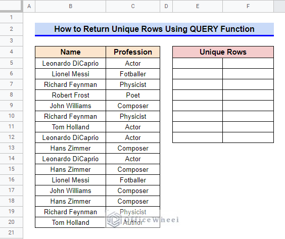
First, let’s get familiar with our dataset. The dataset contains a list of names and professions of a few people. As you can see, several rows have been repeated here. Now, we’ll use the QUERY function to return only the unique rows. So, let’s get started.
1. Combining QUERY and UNIQUE Functions
We can combine the UNIQUE function with the QUERY function to return the unique rows. The UNIQUE function can return a set of unique rows in the order in which they appear in the provided range. We’ll use the QUERY function to return any specified range for the UNIQUE function.
Steps:
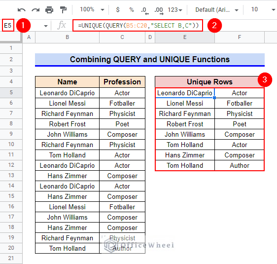
- Firstly, select Cell E5.
- Afterward, type in the following formula-
=UNIQUE(QUERY(B5:C20,"SELECT B,C"))- Finally, press Enter key to get the required result.
Formula Breakdown
- QUERY(B5:C20,”SELECT B,C”)
First, the QUERY function runs a Google Visualization API Query Language query across the range B5:C20. The expression SELECT starts a query. Since we want to provide the entire range B5:C20, we have simply selected columns B and C using the QUERY function. You may run any special query to provide a specified range.
- UNIQUE(QUERY(B5:C20,”SELECT B,C”))
Later, the UNIQUE function returns only the unique rows from the data range returned by the QUERY function.
Read More: How to Get Unique Values Without Blanks in Google Sheets
2. Merging QUERY and ARRAYFORMULA Functions
If we require the frequency count of each row in the data range using the QUERY function, then we have to use the ARRAYFORMULA function along with it. However, all the elements in a row will be merged in a single cell in this method.
Steps:
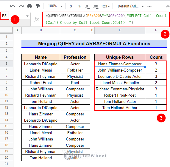
- To start, activate Cell E5 by double-clicking on it.
- Then insert the following formula-
=QUERY(ARRAYFORMULA(B5:B20&"-"&C5:C20),"SELECT Col1, Count (Col1) Group by Col1 label Count(Col1)''")- After that, get the required output by pressing the Enter key.
Formula Breakdown
- ARRAYFORMULA(B5:B20&”-“&C5:C20)
Firstly, the ARRAYFORMULA function merges the subsequent cells of range B5:B20 and C5:C20 with a delimiter “–”.
- QUERY(ARRAYFORMULA(B5:B20&”-“&C5:C20),”SELECT Col1, Count (Col1) Group by Col1 label Count(Col1)””)
Now, the QUERY function runs a Google Visualization API Query Language query across the range returned by the ARRAYFORMULA function. The expression SELECT starts a query. Here the Col1 statement indicates the first column of the provided range. Since the range returned by the ARRAYFORMULA function has only one column, the query performed by the QUERY function will count the frequency of each row in the range and later return it for each row as a group.
Read More: How to Count Unique Values in Multiple Columns in Google Sheets
3. Uniting ARRAYFORMULA, SPLIT, and QUERY Functions
Now, if you don’t require the frequency count of each row in the data range, you can use the SPLIT function along with another ARRAYFORMULA and QUERY function to return the list of unique rows.
Steps:
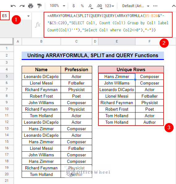
- Select Cell E5 first and then activate it by using function key F2.
- Afterward, insert the following formula-
=ARRAYFORMULA(SPLIT(QUERY(QUERY(ARRAYFORMULA(B5:B20&"-"&C5:C20),"SELECT Col1, Count (Col1) Group by Col1 label Count(Col1)''"),"Select Col1 where Col2<>0"),"-"))- Now, press Enter key to get the required output.
Formula Breakdown
- ARRAYFORMULA(B5:B20&”-“&C5:C20)
First, the ARRAYFORMULA function merges the subsequent cells of range B5:B20 and C5:C20 with a delimiter “–”.
- QUERY(ARRAYFORMULA(B5:B20&”-“&C5:C20),”SELECT Col1, Count (Col1) Group by Col1 label Count(Col1)””)
Afterward, this QUERY function runs a Google Visualization API Query Language query across the range returned by the ARRAYFORMULA function. The expression SELECT starts a query. Here the Col1 statement indicates the first column of the provided range. Since the range returned by the ARRAYFORMULA function has only one column, the query performed by the QUERY function will count the frequency of each row in the range and store it in a new column (Col2).
- QUERY(QUERY(ARRAYFORMULA(B5:B20&”-“&C5:C20),”SELECT Col1, Count (Col1) Group by Col1 label Count(Col1)””),”Select Col1 where Col2<>0″)
Now, this QUERY function will run another query to select and return the rows from Col1 for which the subsequent count is not 0 in Col2.
- SPLIT(QUERY(QUERY(ARRAYFORMULA(B5:B20&”-“&C5:C20),”SELECT Col1, Count (Col1) Group by Col1 label Count(Col1)””),”Select Col1 where Col2<>0″),”-“)
At this time, the SPLIT function divides the merged text around the delimiter “–”.
- ARRAYFORMULA(SPLIT(QUERY(QUERY(ARRAYFORMULA(B5:B20&”-“&C5:C20),”SELECT Col1, Count (Col1) Group by Col1 label Count(Col1)””),”Select Col1 where Col2<>0″),”-“))
Finally, this ARRAYFORMULA function helps the non-array function SPLIT to deal with an array.
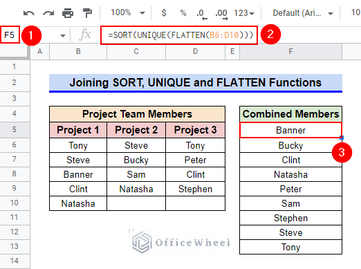
4. Joining SORT, UNIQUE, and FLATTEN Functions
Sometimes, we require finding unique cells from multiple columns in Google Sheets. In such scenarios, we can combine the UNIQUE and FLATTEN functions to return the unique cells in a separate column. Here, we’ll return the unique project member names from the following dataset and sort them using the SORT function.
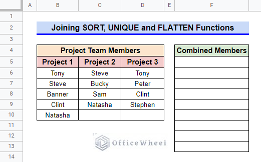
Steps:
- Firstly, select Cell F5 and then insert the following formula-
=SORT(UNIQUE(FLATTEN(B6:D10)))- Finally, get the required output by pressing the Enter key.
Formula Breakdown
- FLATTEN(B6:D10)
First, the FLATTEN function returns all values from the entire range to a single column.
- UNIQUE(FLATTEN(B6:D10)
Afterward, the UNIQUE function returns all the unique rows from the flattened range.
- SORT(UNIQUE(FLATTEN(B6:D10)))
Finally, the SORT function returns a sorted list of unique names.
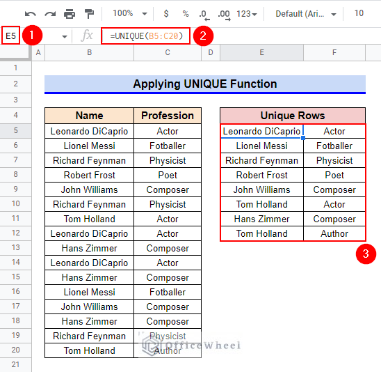
Alternative to Apply QUERY Function for Unique Rows in Google Sheets
Although the QUERY function can return unique rows from the entire range, the amount of work required for it is very tedious in some cases. So when you are searching for a simpler way then you can use the UNIQUE function.
Steps:
- First, activate Cell E5 by double-clicking on it.
- Now, insert the following formula-
=UNIQUE(B5:C20)- Consequently, press the Enter key to get the required output.
Things to Be Considered
- All the elements of a row need to be merged into a single cell before we apply the QUERY function to count the frequency of each row in a data range.
- The UNIQUE function requires a flattened range if we want it to return unique cells from multiple columns.
Conclusion
This concludes our article to learn how to return unique rows using the QUERY function in Google Sheets. I hope the demonstrated examples were ideal for your requirements. Feel free to leave your thoughts on the article in the comment box. Visit our website OfficeWheel.com for more helpful articles.
Related Articles
- How to Filter Unique Values in Google Sheets (5 Simple Ways)
- Use COUNTIF Function to Count Unique Values in Google Sheets
- How to Use Pivot Table to Count Unique Values in Google Sheets
- Find Unique Values in Google Sheets (5 Simple Ways)
- How to Highlight Unique Values in Google Sheets (9 Useful Ways)
- Remove Unique Values in Google Sheets (2 Suitable Ways)