How to Filter Based on a Cell Value in Google Sheets (2 Easy ways)

Cell references can be a huge deal when it comes to automating many spreadsheet features, including filtering. Keeping that in mind, in this article we will focus on how to perform a filter based on the value of a different cell in Google Sheets.

To this end, we can use both the FILTER function and the default filter feature of Google Sheets.

Let’s get started.

2 Ways to Filter Based on a Cell Value In Google Sheets

1. Using the FILTER function to Filter based on a Cell Value in Google Sheets

Cell references are easiest to use with functions and formulas. And when it comes to filtering, the FILTER function is a great one to use.

The FILTER function syntax:

Now, let’s consider the following worksheet:

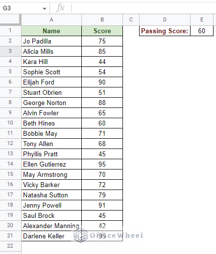
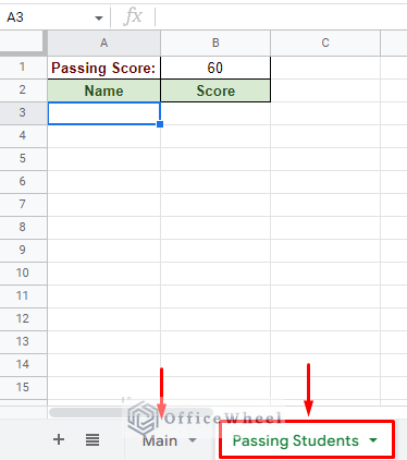
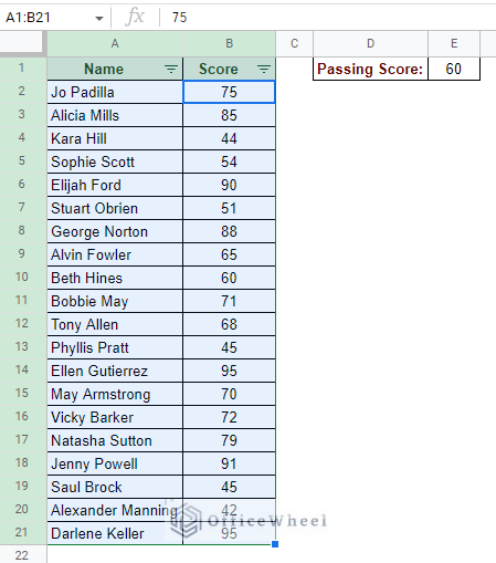
Here, we have the Names and Scores of students and the Passing Score required in a separate cell.

For this example, we will filter the student data based on the Passing Score cell value in Google Sheets.

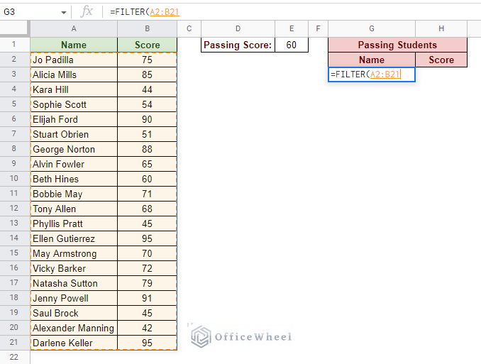
Step 1: Open the FILTER function in the desired cell. Input the data range for the formula.

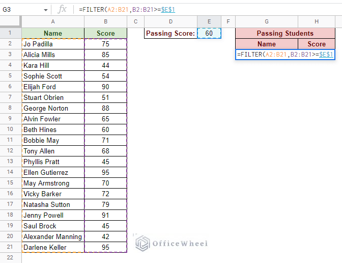
Step 2: Enter the filter condition. In this case, the values of the Score column that are greater than or equal to 60. We will use the reference Score from cell E1.

Note that we have locked the cell reference with an absolute ($) to make the formula always refer to cell E1. Tip: Press the F4 key of the keyboard to cycle through different cell locks.

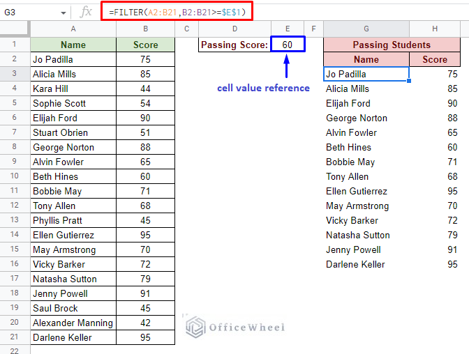
Step 3: Close parentheses and press ENTER.

Does Not Contain Value (Match Text Example)

If you didn’t already know, we can also use the FILTER function to filter by text values in Google Sheets.

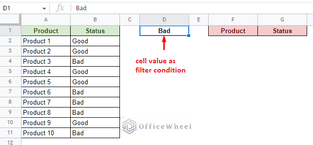
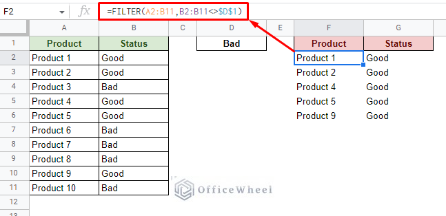
In this example, the filter condition is dependent on the value in a different cell, cell D1. Not only that, we will spice things up by filtering for all entries that do not contain that text value.

We once again reference the cell that contains the filter condition for the FILTER formula:

We used the “not equal to” symbol (<>) to achieve the “does not contain” criteria. Again, we have locked the cell value reference with absolutes ($).

For multiple text criteria using both AND and OR logic, please see this article: Google Sheets: Filter for Multiple Criteria with Formula (2 Easy Ways)

From Another Worksheet

It is always a good idea to keep spreadsheets organized. A common way to do this is by using multiple worksheets.

While many features might have a problem with data scattered around different places, cell references easily overcome this for functions like FILTER.

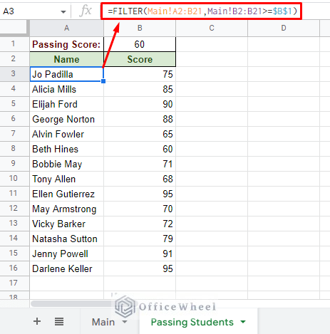
For this example, we will once again apply the first method, only this time the filter will be presented in a separate worksheet.

If we analyze the scenario, we will see that only the source data range is in a separate worksheet. That is where the filter values come from. So, the updated formula is:

Read More: Filter Entries if it Does Not Contain Value in Google Sheets (2 Easy Ways)

Similar Readings 

• How to Use Data Validation and Filter in Google Sheets (4 Ways)
• Filter with QUERY for Multiple Criteria in Google Sheets (An Easy Guide)
• How to Filter with the OR Condition in Google Sheets (3 Easy Ways)
• Delete Filter Views in Google Sheets (An Easy Guide)
• How to Create Filter Views in Google Sheets (An Easy Guide)

2. Using the Default Filter Feature of Google Sheets to Filter Based on Cell Value

The default filter does not allow users to apply cell references to any of the conditions in the menu.

To do so, we must apply a custom formula to this menu.

Step 1: Apply a filter over the source data range.

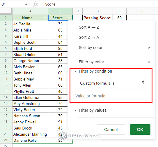
Step 2: Navigate to the “Custom formula is” option in the filter menu.

Filter > Filter by condition > Custom formula is

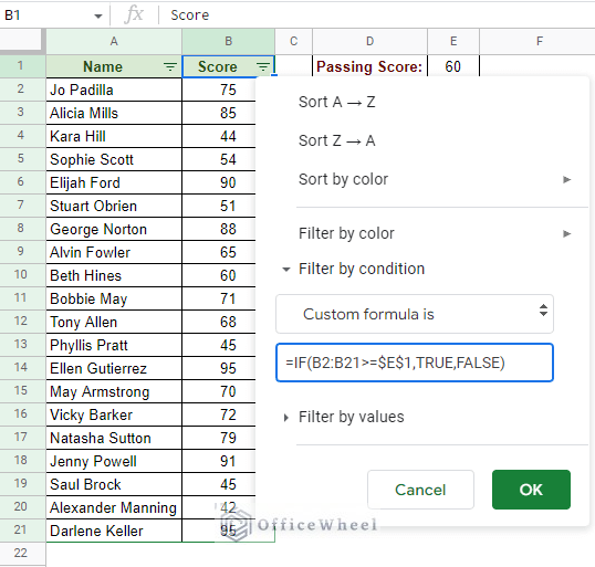
Step 3: Apply the following custom formula in the field:

The formula follows the same logic as we saw for the FILTER function.

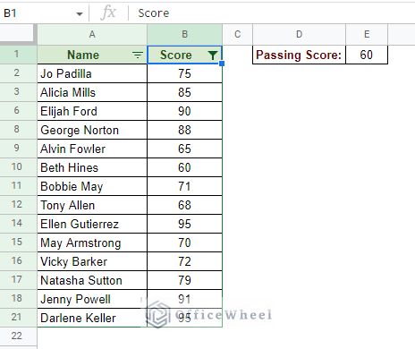
Step 4: Click OK to apply the filter for values greater than the value in cell E1 in the Google Sheets worksheet.

Read More: How to Filter by Condition Using a Custom Formula in Google Sheets (3 Easy Examples)

Final Words

That concludes the two ways we can filter based on a cell value in Google Sheets. Among them, we prefer using the FILTER function method as it allows us to further customize the filter condition much more easily.

Feel free to leave any queries or advice you might have for us in the comments section below. Or have a look at some of our other related articles that are sure to interest you.

Related Articles

• How to Find and Replace Blank Cells in Google Sheets
• Use Wildcard in Google Sheets (3 Practical Examples)
• How to Filter By Rows in Google Sheets (An Easy Guide)
• Filter with the AND Condition in Google Sheets (An Easy Guide)
• How to Filter for Multiple Conditions in Google Sheets (2 Easy Ways)
• Applying Filter with REGEXMATCH Function in Google Sheets (Easy Examples)
• Filter Data Using Filter Views in Google Sheets (An Easy Guide)
• Google Sheets: Filter Data if it Contains Value (A Comprehensive Guide)