How to Lock Cells with Formula in Google Sheets (with Easy Steps)

Suppose you are working on a sensitive dataset for your company. The information of the dataset belongs to a particular department. In that case, locking the sheet or the cells of the dataset is a smart move. Otherwise, someone can delete the information accidentally. Here, we will learn how to lock cells in google sheets formula step by step.

The overview of this article is above. You will learn more about this article once you go through the total article. So, let’s start.

Table of Contents

A Sample of Practice Spreadsheet

You may copy the spreadsheet below and practice by yourself.

Lock Cells with Formula

Step By Step Procedures to Lock Cells with Formula in Google Sheets

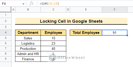
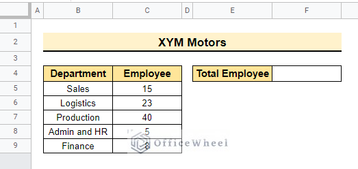
The dataset contains Employee and Department. That represents the employee number in each department. We need the total number of employees. After getting the sum of the total employees now we will lock the formula cell F4 so that the other people cannot change the value using the dataset. Once we lock the cell without the owner and the editor no other person will have the access to edit the cell. Other people have viewer access only.

Step 1: Selecting Dataset Range

Here, we will process the dataset so that we can lock the selected range. So follow the below steps to execute this process.

Initially, select cell F4 to lock the cell.
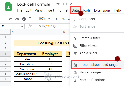
After that, select Data >> Protect sheets and ranges to protect the particular cell.

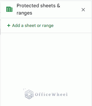
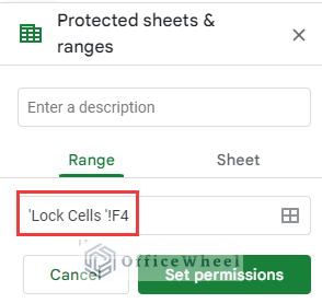
Protected sheets & ranges window will pop up to select the range.

Step 2: Setting Permission

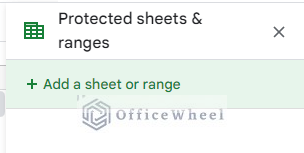
Therefore, select add a sheet or range to add the sheet range and as cell F4 is already selected this cell will show as the referred range.

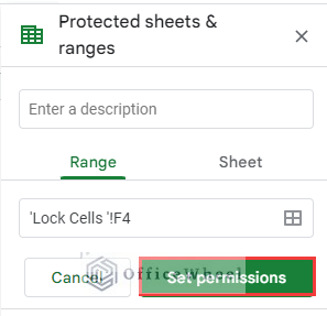
Moreover, select Set permissions to set the editor and viewer of the cells.

Step 3: Locking Formula Cells

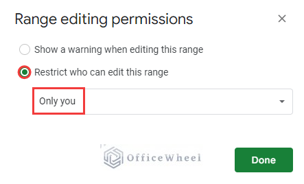
Afterward, the Range editing permissions window will appear
Consequently, you can see Restrict who can edit this range and Only you is selected by default.

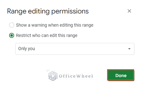
Now, click Done to complete the method.

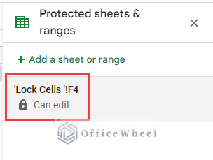
Finally, the selected range will appear in the Protected sheets & ranges window.

How to Lock Cell Reference in Google Sheets While Using Formula

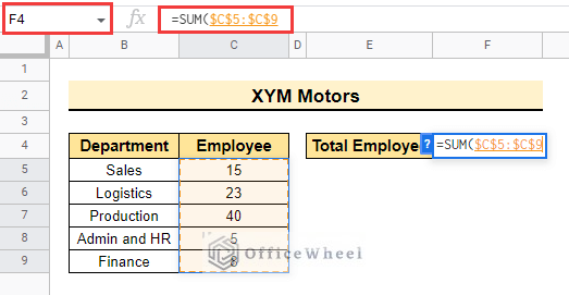
The dataset contains Department and Employee. The dataset contains the employee numbers of individual departments. Let’s sum up the number of employees and while doing this we will lock the cell reference so that the cell reference doesn’t change. Say, you need to copy a specific formula in your dataset. Here if you drag down the fill handle and copy the formula in every blank cell then the cell reference will change according to the number of the column (Suppose the reference is C5 in the formula. But if you drag down the Fill handle and paste the formula into cell D6 then the cell reference will be C6 in the formula). But if you lock the cell reference before dragging down the fill handle then the formula will remain the same and this will save you time and double work. So, follow the steps below to execute this process.

📌 Steps:

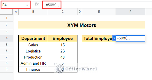
First, select cell F4 and enter the SUM function to execute this formula.

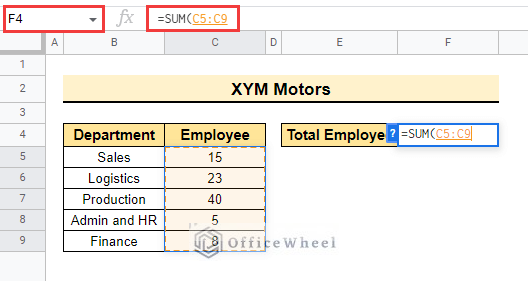
Then, select range C5:C9 to complete the process and get the result.

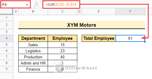
After that, lock the cell reference by pressing the F4 key or by putting a dollar sign ($) beside the row and column number of the cell references. So that the result remains constant after pasting this formula into another cell.

Finally, the result will be the same and secure after copying this formula and paste it to another cell.

Once you lock the cell reference then you can copy and paste the formula into another cell but eventually, the cell reference will show C5:C9 as the reference is already locked.

How to Edit Permission of Locked Cells with Formula in Google Sheets

You can also edit permission after you selected only me. The steps are shown below with the following dataset. Follow the steps below to do this.

📌 Steps:

Initially, repeat the steps above to get the Protected sheets & ranges window.
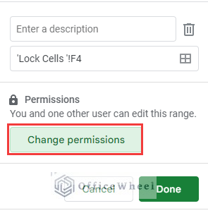
Afterward, click Change permissions from Protected sheets & ranges window.

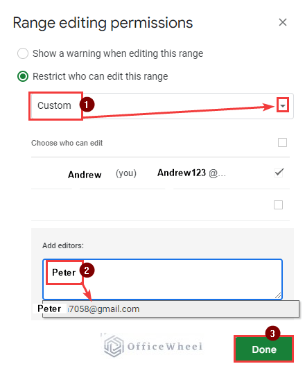
And again Range editing permissions window will pop up. Then select Custom instead of Only me from the dropdown and enter the email account of the editor in the Add editors: group.
After that, complete the process by clicking Done.

Things to Remember

Only the sheet owner or the editor can edit the protected sheets.
You can also lock the total sheet from Protect sheets window so that the viewer cannot edit any cells.

Conclusion

In this article, we explained how to lock cells in google sheets formulas step by step. Hopefully, this procedure will help you apply this method to your dataset. Please let us know in the comment section if you have any further queries or suggestions. You may also visit our OfficeWheel blog to explore more Google Sheets-related articles.