Google Sheets makes it simple to work with coworkers on the same spreadsheets with its simple sharing features. Although working on the same spreadsheet is so simple, it’s also easy for a user to change important equations that the spreadsheet depends on. A single action might destabilize the entire sheet. The good news is that Google Sheets allows you a lot of flexibility regarding user permissions to protect formulas. The Protected sheets and ranges tool prevents any alteration of a cell or range of cells and also offers other customized settings. In this article, I’ll demonstrate 2 quick ways to protect the formulas in Google Sheets. Here is an overview of what we will achieve:
2 Quick Ways to Protect Formulas in Google Sheets
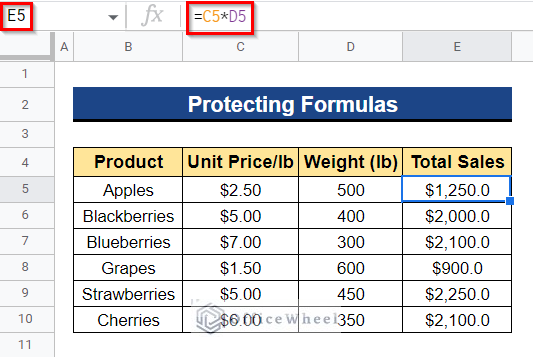
We will use the dataset below to demonstrate 2 quick ways to protect the formulas in Google Sheets. The dataset contains a list of products, their unit prices per pound, the total weight of each product, and the total sales of each product of a particular shop. Here, the unit price per lb of each product is multiplied by the product weights to determine the total sales of each product. Now, we want to protect the formula of the total sales, so that no one will be able to make changes to the formula.
1. Warning Users Before Editing
You may wish to warn users before editing the spreadsheet. As a result, the users will get notified when they try to make changes to the spreadsheet. In our dataset, we wanted to protect the formula of the total sales. So we can show a warning using this example if any one of the users tries to modify the value in the total sales column.
Steps:
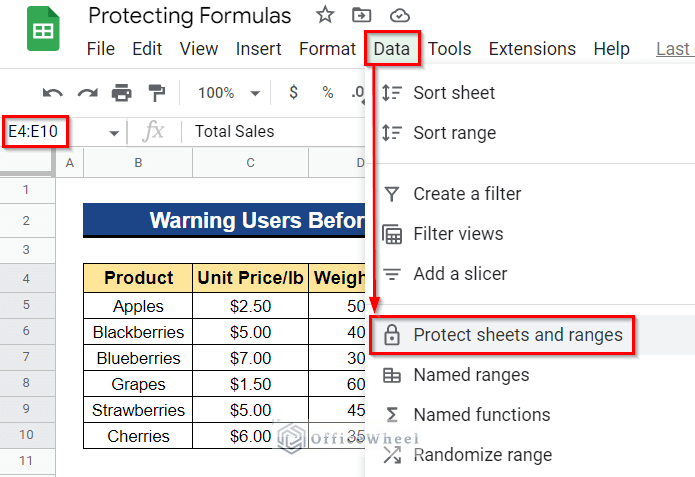
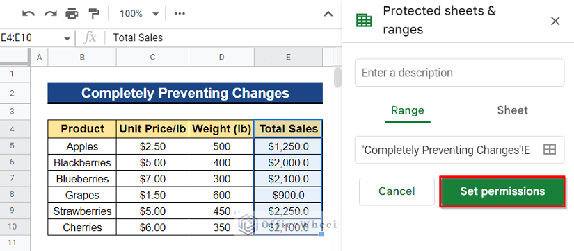
- Firstly, select the cell range that you wish to protect. In our case, we selected Cell E4:E10. Next, go to the Data tab from the top menu bar and select Protect sheets and ranges.
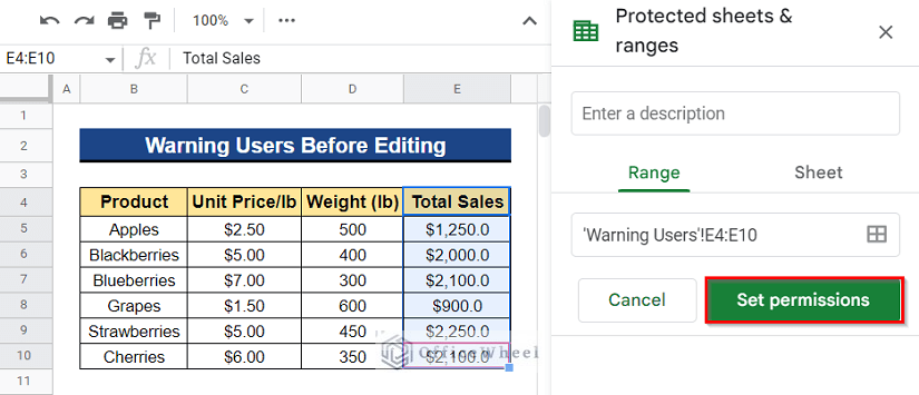
- As a result, a dialog box titled Protected sheets and ranges will appear on your screen.
- Now, click Set permissions.
- As a consequence, it will appear permission rules for the cell range.
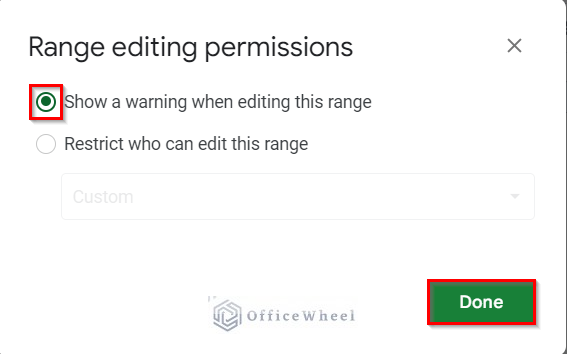
- Next, if you want to warn users before editing, click on Show a warning when editing this range and then select Done.
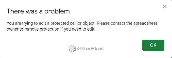
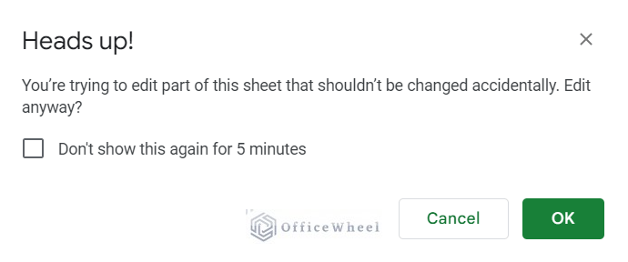
- Therefore, the notification below will appear whenever one of your coworkers tries to alter the value of the chosen data range.
Read More: Protect Range in Google Sheets (Easy Examples)
2. Completely Preventing Changes
Instead of displaying warnings before editing, you could want to totally restrict alteration to the chosen data range. The users will be alerted when they attempt to modify the spreadsheet as a consequence, and they won’t be allowed to modify the data range without your permission.
2.1 For All Users
You may wish to restrict all users from editing the selected cell range of the datasheet. As a result, all users won’t be able to make modifications to the selected cell range without your permission.
Steps:
- Choose the cell range that you want to protect first. In this instance, we chose Cell E4:E10.
- Next, select Protect sheets and ranges from the Data tab in the top menu bar.

- As a result, your screen will display a dialog box with the title Protected sheets and ranges.
- Click Set permissions after that.
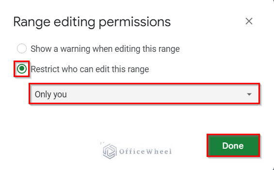
- Permissions for the cell range will therefore be shown. Next, to restrict users, select Restrict who can edit this range.
- Then choose Only me from the drop-down list before selecting Done if you want to prevent any of the users from making changes to the specified cell range.
- As a result, if one of your coworkers tries to change the value of the selected data range, the notification below will show up and they won’t be able to make changes.
Read More: How to Lock Cells with Formula in Google Sheets (with Easy Steps)
2.2 For Certain Users
You might want to prevent everyone except specific users from modifying the datasheet’s specified cell range. Users excluding some specific users won’t be able to change the chosen cell range without your approval as a consequence.
Steps:
- First, decide which cell range you want to protect. In this case, we chose Cell E4:E10.
- Afterward, select Protect sheets and ranges from the Data tab in the top menu bar.
- As a result, a dialog box with the title Protected sheets and ranges will show up on your screen.
- Next, click Set permissions.
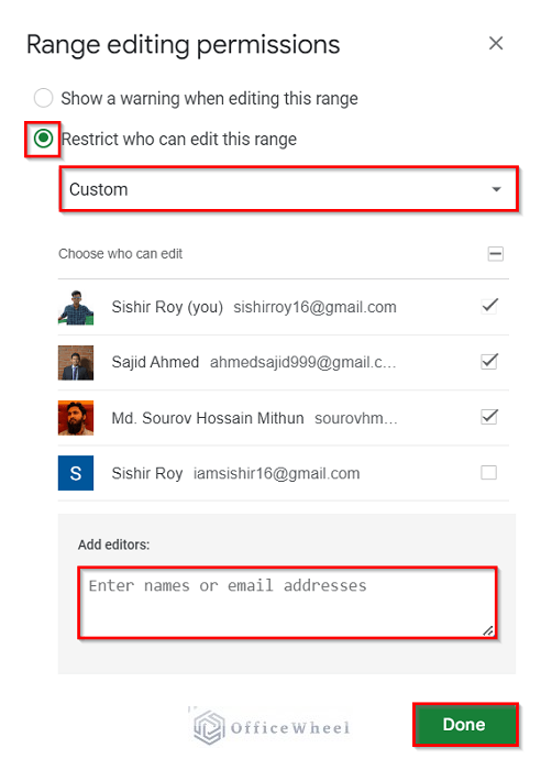
- As a result, the cell range’s permission rules will be shown. To restrict users, click Restrict who can edit this range next.
- Furthermore, pick Custom from the drop-down box if you wish to limit users by excluding certain users from making changes to the specified cell range. It will display the access permissions for this cell range.
- In the Add editors section, you may add editors by their names or email addresses to the specified cell range. Finally, click Done.
- Therefore, the message below will appear and they won’t be able to make changes if one of your coworkers, except the designated users, tries to modify the value of the chosen data range.
Read More: How to Lock Cells in Google Sheets (4 Ways)
Conclusion
This brings up an end to this article. Here, I’ve covered 2 simple examples to protect the formulas in Google Sheets. I hope this will meet your requirements. Please feel free to any queries or suggestions in the comment section below. To explore more of these informative articles on Google Sheets, visit our website Officewheel.com.