You can never get enough protection for your crucial spreadsheets. To that end, we believe, you can’t get any safer than the conditional locking of cells in Google Sheets.
And that is what we will be looking at today. So, let’s get started.
Conditionally Locking Cells in Google Sheets in Two Easy Steps
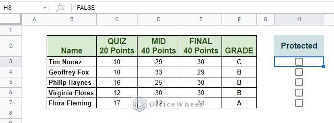
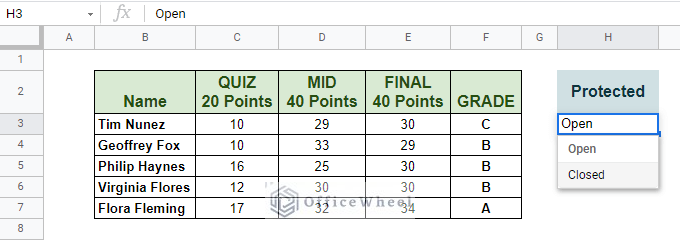
To show our process, we will be going to use the following dataset:
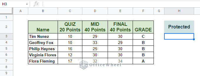
Here, we want to lock the values of columns Quiz, Mid, and Final, so that the scores can’t be edited unless permitted.
We will be showing you two separate types of conditions for Protection simultaneously:
- Checkbox
- Drop-down menu
Step 1: Set Up the Condition Via Data Validation
I. Using Checkbox
First of all, we set up the Protected condition with a checkbox. The idea is if the checkbox is ticked (TRUE) then the range of cells will be locked.
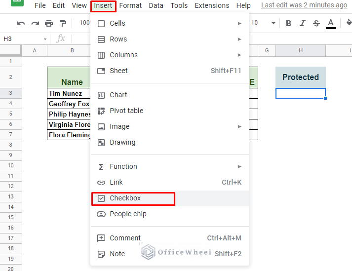
To insert a checkbox, simply select the cell where you want it and navigate to it from the Insert tab. Insert > Checkbox
Once the checkbox is in place, we can move to the Data Validation steps to lock our cells.
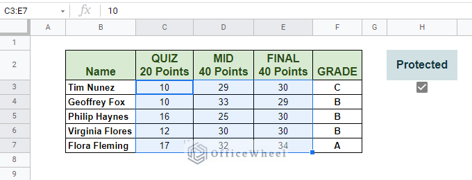
1: Select the range of cells that you want to apply Data Validation to. For us, they are the value cells of Quiz, Mid, and Final, cells C3:E7.
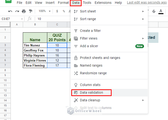
2: Navigate to Data Validation from the Data tab. Data > Data validation
3: In the Data validation window, select the Custom formula is option from the drop-down in the Criteria section. We must define a custom formula for our condition.
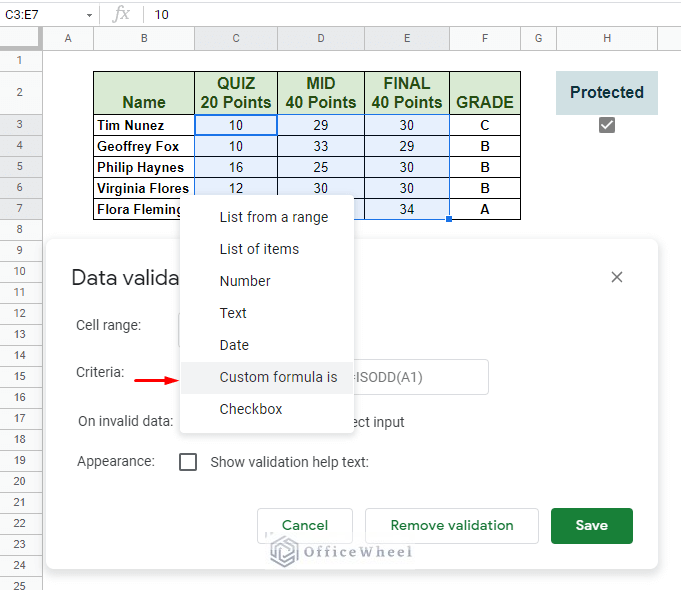
4: Apply the following custom formula:
=$H$3=FALSE5: Check the Reject input radio button
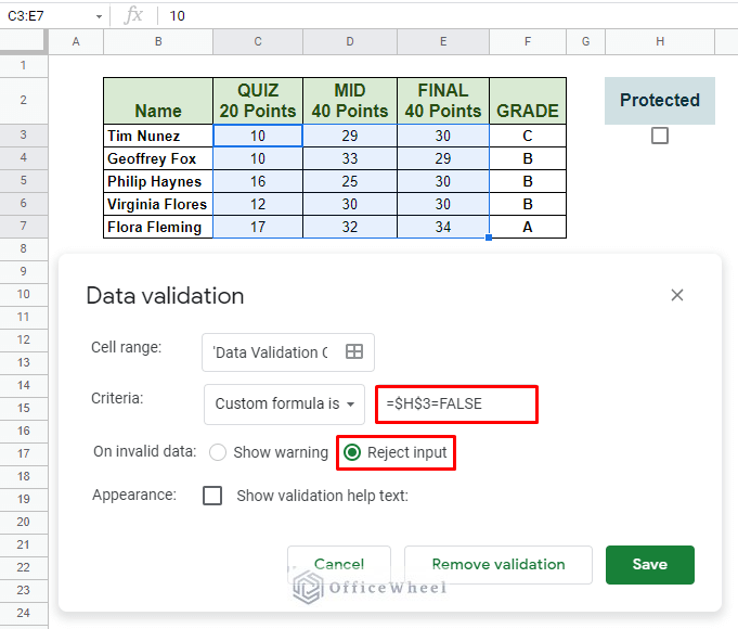
What points 4 and 5 does: As long as our checkbox in our worksheet (at cell H3) is TRUE, the Data validation will reject any input to the selected cells. The condition cell reference is locked by absolutes ($) so that the formula does not move with each cell in the data validation selection.
6: Click Save.
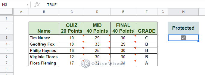
The process in action:
If you want to apply a lock to each row, simply add a checkbox to each row:
And change the custom formula to:
=$H3=FALSE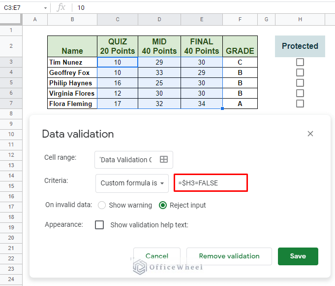
Note: We have removed the absolute ($) from the row reference to free it up as the condition moves to each new row. This is called a mixed cell reference.
Read More: How To Lock Rows In Google Sheets (2 Easy Ways)
II. Using Drop-Down Menu
Using conditions from a drop-down menu is as simple as the checkbox method. Only this time, our options of protection will be listed in a drop-down menu.
On the same dataset, create a drop-down menu with the two conditions, Open and Closed. We do this, coincidentally, by using the Data validation option.
In cell H3 we apply the following data validation:
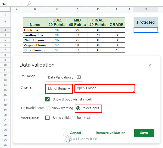
- Criteria: List of items
- Options: Open, Closed
- Reject Input
The only thing we are going to change now from the previous Data validation condition is the custom formula.
=$H$3="Open"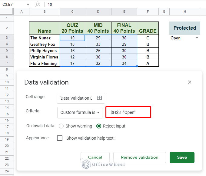
The result:
Read More: How to Lock Cells with Formula in Google Sheets (with Easy Steps)
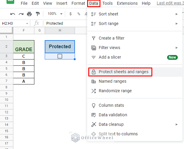
Step 2: Protect Your Condition Cells With The Protect Range Option
Our process is still incomplete since anyone can enter and switch our conditions in the Protected column to edit the locked cells. We need another layer of protection that allows only us, and certain collaborators, to be able to change the locked conditions.
We do this by using the Protect Range option of Google Sheets.
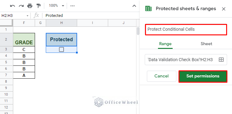
1: Select the condition cells and navigate to the Protect sheets and ranges option from the Data tab.
2: Name your locked range [Optional] and click on Set permissions.
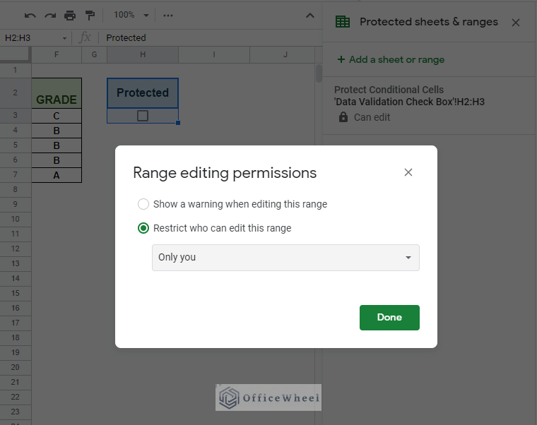
3: We leave the Permission as Only you and then click Done.
We have successfully locked the condition cells of our worksheet. Now, if anyone tries to change the conditions other than us, they will be hit with the following warning:
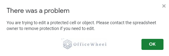
On top of having a conditional lock on the value cells.
Please read our How to Lock Cells in Google Sheets article for an in-depth guide on how to use the Protect Range option to lock cells.
Read More: Protect Range in Google Sheets (Easy Examples)
Final Words
That concludes the method for conditional locking of cells in Google Sheets. We hope that now you can apply this unorthodox yet simple procedure to your spreadsheets.
Please feel free to leave us any queries or advice you might have in the comment section.