Today, we will look at how to lock a column in Google Sheets in the most basic way available to us in the application.
As an extra situational example, we will also explore how to lock columns conditionally later in the article. So let’s get started.
How to Lock a Column in Google Sheets
The Basic Way to Lock a Column in Google Sheets
We start with the fundamental way to lock any cell or column in Google Sheets, that is, by using the Protect Range option.
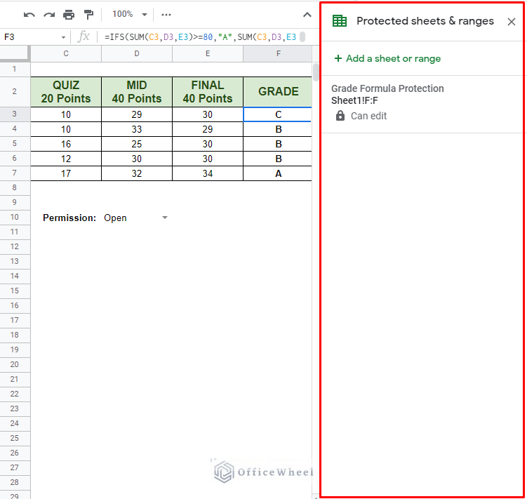
And for our example, we will be using the following worksheet:
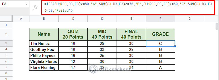
Notice that the Grade column contains a formula. Thus, it is crucial to lock this particular column to protect it from alterations.
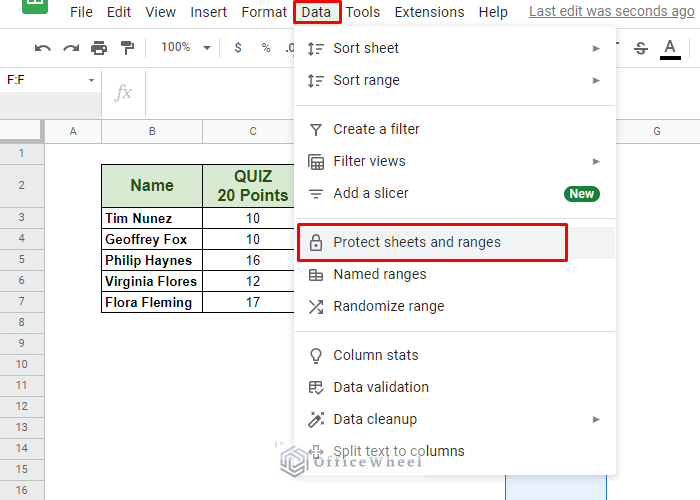
Step 1: Select the column (we have selected the whole column) and open the Protect range menu. We can navigate to Protect range in two ways:
1. From the Data tab. Data > Protect sheets and ranges
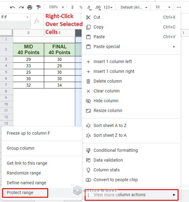
2. Right-clicking over the selected cells. Right-click > View more column actions > Protect range
This should open the Protected sheets & ranges menu
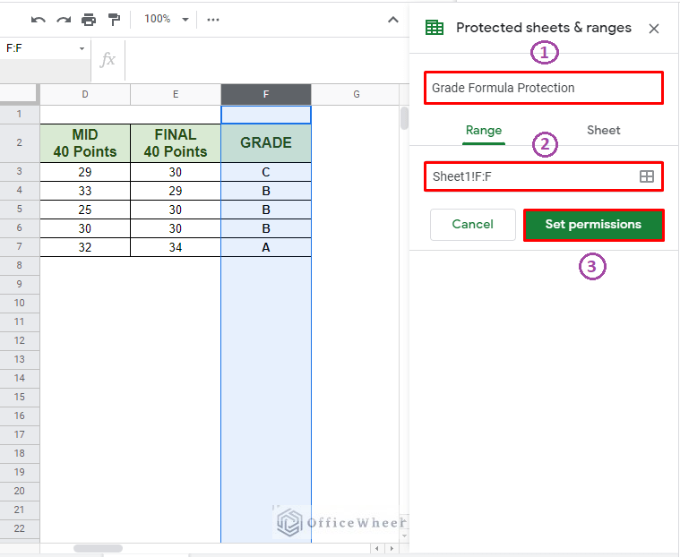
Step 3: Here we have three sections to note:
- Naming the protected range [Optional]. You can name your locked cells for better organization.
- Range of protected cells which will be locked from further changes. You can change the range again from here.
- Click Set permissions to move to the next step.
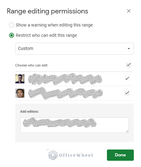
Step 3: By default, you will be presented with the following Range editing permissions window:
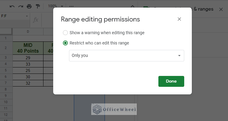
For now, we have restricted the permissions only to us. Click Done to apply the lock.
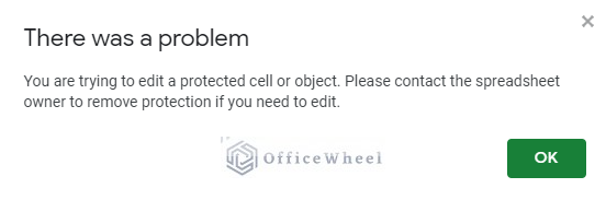
Now, if anyone else goes to change anything within the locked column, they will be hit with the following message:
Points to Note:
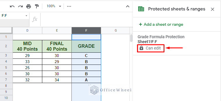
- If the Can edit message appears in the Protected sheets & ranges menu, you have permission to edit the locked cells in this worksheet. Otherwise, you can’t.
- You can choose to select Custom permissions in the Range editing permissions window to add more people to edit the locked cells in Google Sheets.
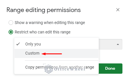
Select Custom Permissions
Adding more people to collaborate
You can read our How to Lock Cells in Google Sheets article for an in-depth guide.
Read More: Protect Range in Google Sheets (Easy Examples)
How to Conditionally Lock a Column in Google Sheets
We can use the Protect range option to lock any range of cells we desire. But what if we want to lock cells if they meet a particular criterion?
We cannot add conditions to the Protect range option, however, we can use another function in Google Sheets called Data Validation to do so.
The Data validation option allows us to add a custom formula as criteria in Google Sheets.
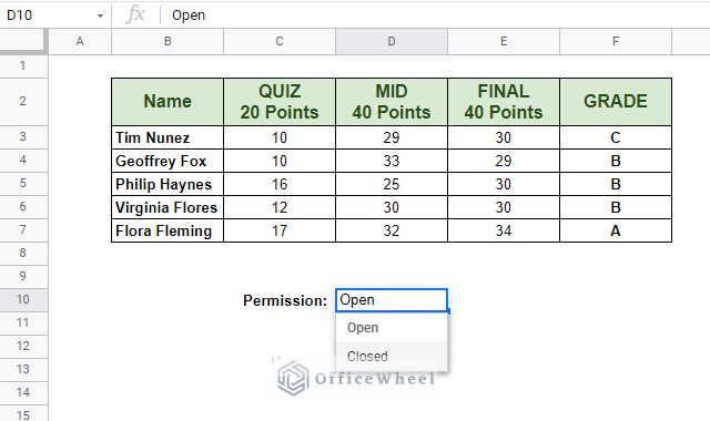
To show this process, let’s transform our existing worksheets to follow this scenario:
You are a supervisor to teachers. Depending on your permission, you can either Open or Close the range of cells containing the points of students for others to edit. Note that the Grade column is already locked.
So, let’s first add a drop-down for the Open or Closed permissions.
Steps to Lock Columns with Data Validation in Google Sheets
Now we begin the process of locking cells with conditions using Data Validation.
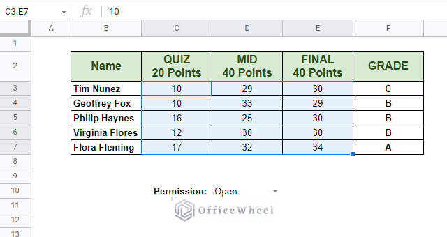
Step 1: Select the range of cells that is to be locked. For us, it’s C3:E7 as we want to lock the Quiz, Mid, and Final columns.
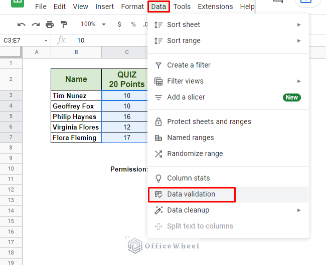
Step 2: Navigate to Data Validation. Data > Data validation
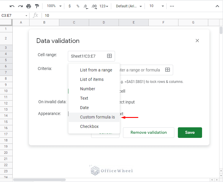
Step 3: Since we are going to define the criteria for locking cells, we will select the Custom formula is option from the Criteria section in the Data validation window.
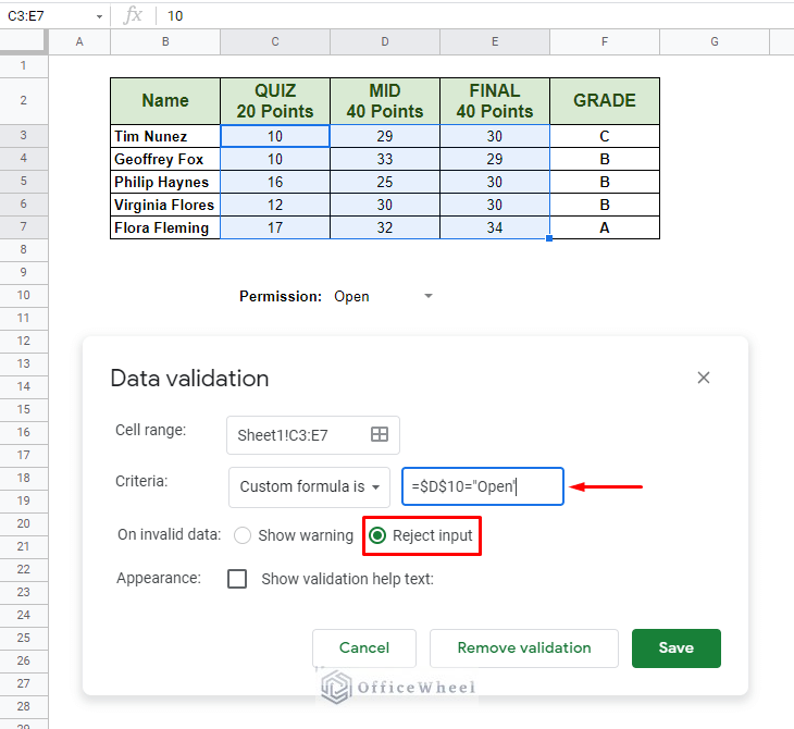
Step 4: Add the custom formula:
Step 5: Check the Reject input radio button in the On invalid data section.
Breakdown:
The Reject input option essentially gives the condition that if cell D10 does not have the value “Open”, you cannot enter or change existing data. We have locked the cell reference D10 with absolutes ($) so that it doesn’t move along with the selected range.
Step 6: Click Save.
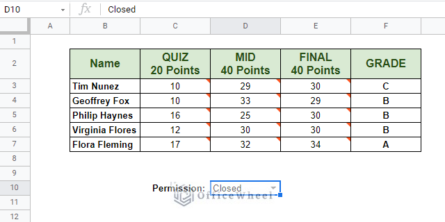
Now anyone is restricted (also gets an error message) from changing the scores in our table as long as we keep the permission Closed.
Additional Step: We have also locked cells C10 and D10 with Protect range so that only we can change the Permission.
Read More: Conditional Locking Of Cells In Google Sheets (Easy Steps)
How to Unlock a Column
Unlocking columns in Google Sheets is as easy as locking them.
With an active locked cell selected, navigate to Protect sheets and ranges from the Data tab. Data > Protect sheets and ranges
If protected cells exist in your worksheet, the Protected sheets & ranges menu should look like this:
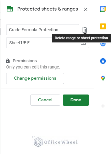
From this menu, you can now select the locked range of cells that you want to edit or remove by simply clicking on it.
Here, click the trash can icon to remove or unlock the locked column.
You will be given a final prompt before removing the locked column.
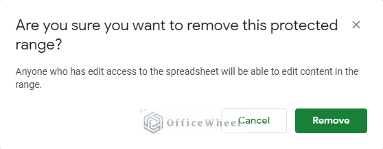
And we are done!
Read More: Protect Sheet From View in a Google Spreadsheet (2 Ways)
Why Do We Need To Lock Cells In Google Sheets?
- You are sharing your workbook with a large audience. Many workbooks are shared publicly but leaving it on view-only mode may not cut it for every situation. You may need certain sheets or certain cells of your workbook to be restricted from third-party edits.
- You may need other users to fill up “input” cells. A form for example, where the user may need to fill up certain fields that apply to them, but not change other important cells or fields that have crucial information in them.
- Specifically, to protect cells that have complex or important formulas. The same applies to references.
Final Words
We hope that the ways of how to lock cells in Google Sheets we have discussed in this article come in handy in your spreadsheet tasks.
Feel free to leave any queries or advice you might have for us in the comment section.