Creating a search box in Google Sheets is helpful for searching for a special piece of information in your spreadsheet and extracting the results in a quick and simple way. Although, the purpose of creating a search box in Google Sheets is not limited to searching for information only. We can apply different filters and unique criteria to the search box while searching for information. So, let’s go through 4 practical methods on how to create a search box in Google Sheets in the next sections.
A Sample of Practice Spreadsheet
4 Easy Methods to Create a Search Box in Google Sheets
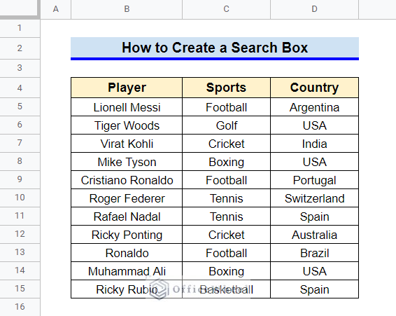
First, let’s get familiar with our datasheet. It contains the names of several famous athletes, the sport they play, and their origin country. We’ll create a search box to search for information from this datasheet. Keep reading to learn how.
1. Applying QUERY Function and Data Validation
Applying the QUERY function along with the Data Validation tool is the most efficient method of creating a dynamic search box in Google Sheets. Although the QUERY function is a bit complex to use, you can easily apply it by following the steps described below.
Steps:
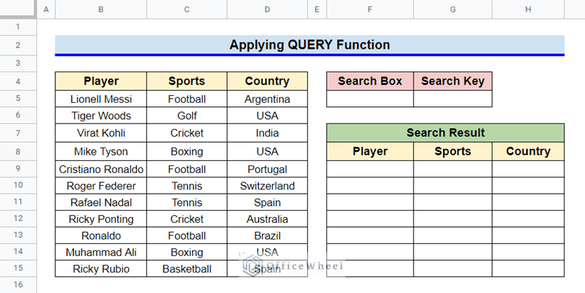
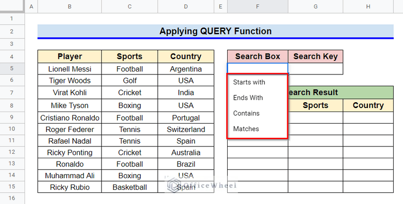
- Modify the datasheet like the following by specifying cells for the Search Box, Search Key, and Search Result.
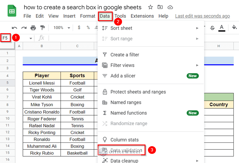
- Now, select Cell F5 and go to the Data From the options, click on Data Validation.
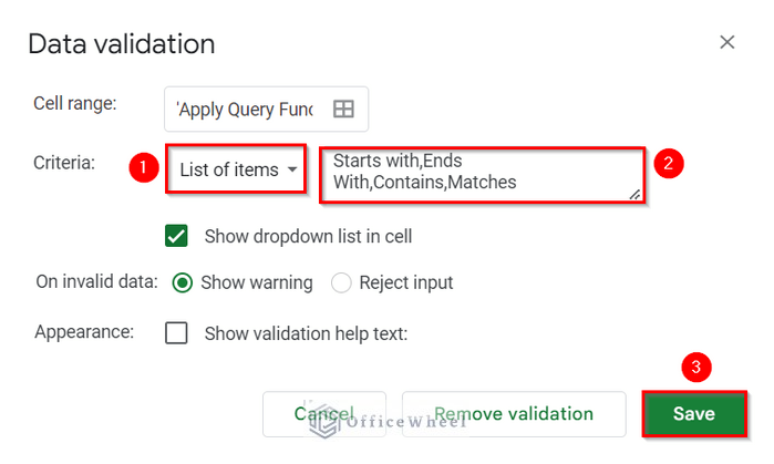
- A window like the following will pop out. Click on the drop-down icon of the Criteria
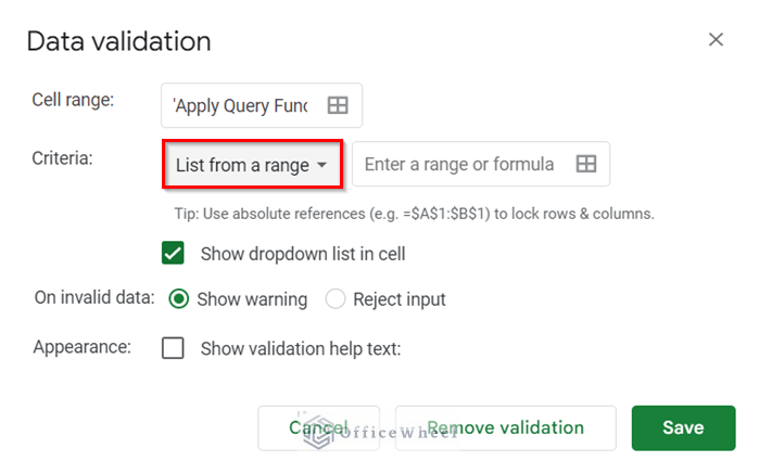
- From the drop-down options, select List of Items, and type in the following list with a Comma (,) symbol between them-
Starts with, Ends With, Contains, Matches.
- Remember to check the grammar of the listed items. The QUERY function won’t work if grammatical errors are present. After that, click on Save.
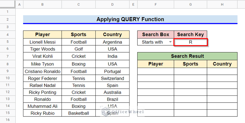
- We have created a drop-down list in Cell F5. Click on the drop-down icon to see the list and choose anyone from the list. I have chosen Starts with.
- Now, insert any search key in Cell G5.
- Finally, select Cell F9, type in the following formula, and press Enter key to get the search result.
=IFERROR(QUERY(B5:D15,"SELECT * WHERE B "&F5&" '"&G5&"' "),"No Match")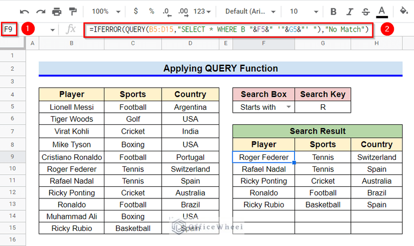
Formula Breakdown
- QUERY(B5:D15,”SELECT * WHERE B “&F5&” ‘”&G5&”‘ “)
First, the QUERY function runs a Google Visualization API Query Language query across the range B5:D15. The expression SELECT * WHERE starts a query. Next expression B indicates the query run in Column B. And the expression “&F5&” indicates the query operator. The & symbols are used for extracting the text from Cell F5. The expression ‘“&G5&”’ indicates the cell reference of the search term. The apostrophes (‘’) symbol differentiates the search term from the search operator.
- IFERROR(QUERY(B5:D15,”SELECT * WHERE B “&F5&” ‘”&G5&”‘ “),”No Match”)
Finally, the IFERROR function returns the value(s) returned by the QUERY function if no error is found. Else, the text “No Match” is returned.
- You can change the search box and search key according to your requirement. Here, we changed to Contains in the Search Box and placed ‘li’ as the Search Key.

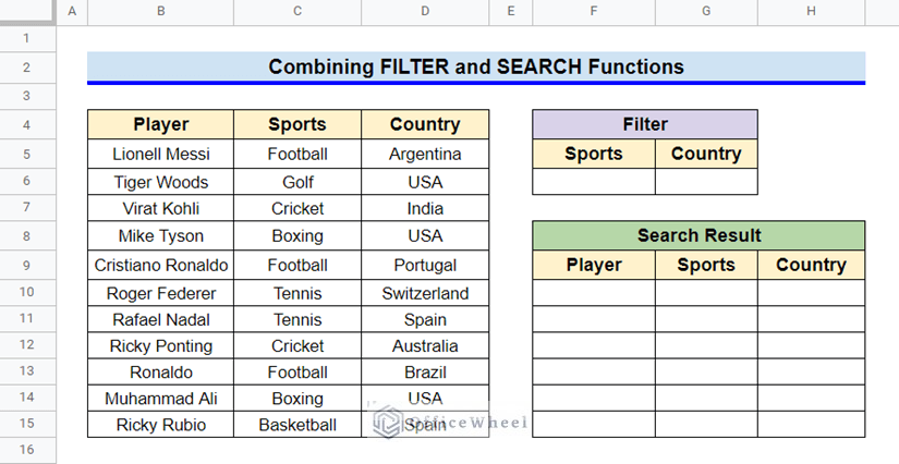
2. Combine FILTER and SEARCH Functions
Another easy method to create a search box in Google Sheets is to combine the FILTER and SEARCH functions in a formula. This method is useful when you want to search for information based on multiple values. Go through the following steps to learn how.
Steps:
- Modify your datasheet like the following by specifying cells for Filter and Search Result.
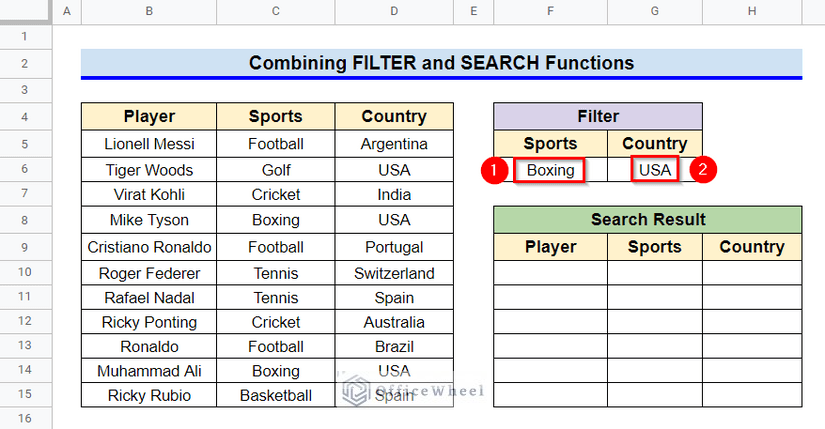
- Then, manually type the filter values in Cell F6 and Cell G6. You can also create a drop-down list if you want.
- Now, select Cell F10, type in the following formula, and then press the Enter key to get the search result-
=IFERROR(FILTER(B5:D15,SEARCH(F6,C5:C15),SEARCH(G6,D5:D15)),"No Match")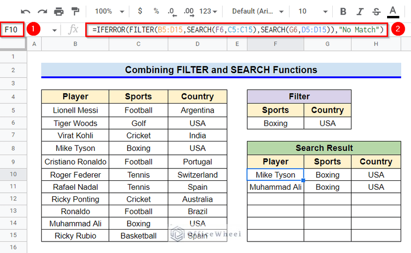
Formula Breakdown
- SEARCH(F6,C5:C15)
Firstly, the SEARCH function returns the position at which the string from Cell F6 is first found within range C5:C15.
- FILTER(B5:D15,SEARCH(F6,C5:C15),SEARCH(G6,D5:D15)
Secondly, The FILTER function returns only the rows which meet the criteria set by the SEARCH functions.
- IFERROR(FILTER(B5:D15,SEARCH(F6,C5:C15),SEARCH(G6,D5:D15)),”No Match”)
Finally, the IFERROR function returns the value(s) returned by the FILTER function if no error is found. Else, it returns the text “No Match”.
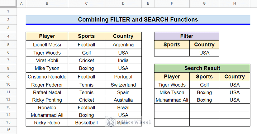
- You can change the filter keys according to your requirements and the search result will change accordingly.
Read More: How to Use SEARCH Function in Google Sheets (5 Examples)
3. Apply MATCH Function
We can also apply the MATCH function to get the relative position of any search key in a specified range. Although, the MATCH function returns the relative position of the first occurrence only.
Steps:
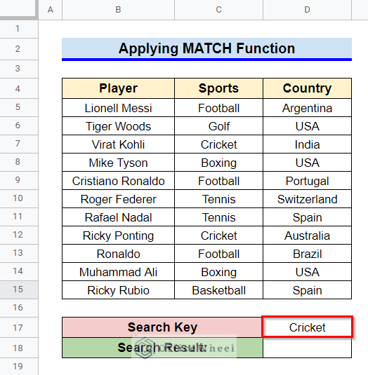
- First, specify cells for the search key and search result. After that, insert the search key in Cell D17.
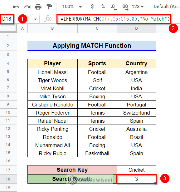
- Now, select Cell D18, type in the following formula, and press Enter key to get the output-
=IFERROR(MATCH(D17,C5:C15,0),"No Match")Soon after, it will return the relative position from the column for the first occurrence.
Formula Breakdown
- MATCH(D17,C5:C15,0)
Firstly, the MATCH function returns the relative position of the first occurrence of the string from Cell D17 in the range C5:C15.
- IFERROR(MATCH(D17,C5:C15,0),”No Match”)
Then, the IFERROR function returns the value returned by the MATCH function if no errors occur. Else, it returns the text “No Match”.
- If you look at the datasheet, in the specified range C5:C15, the search key ‘Cricket’ is in the 3rd and 8th relative positions. The MATCH function has returned the first occurrence.

4. Use FIND Function
The FIND function is useful when one wants to know the relative position of any string within a specified text. The FIND function also returns the relative position of the first occurrence.
Steps:
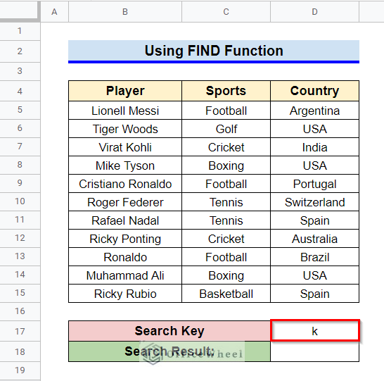
- Firstly, specify cells for the search key and search result. Then, enter your search key in Cell D17. We’ll search for ‘k’.
- Now, select Cell D18 and type in the following formula. And then, press Enter key to get the relative position-
=IFERROR(FIND(D17,B12),"No Match")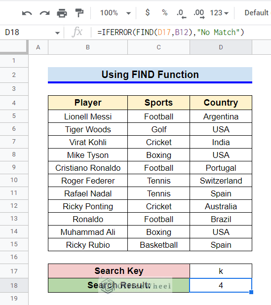
Formula Breakdown
- FIND(D17,B12)
First, the FIND function will return the relative position of the string in Cell D17 within the specified text in Cell B12.
- IFERROR(FIND(D17,B12),”No Match”)
Then, the IFERROR function returns the value returned by the FIND function if no error is found. Else, it returns the text “No Match”.
An Alternate Way to Search in Google Sheets
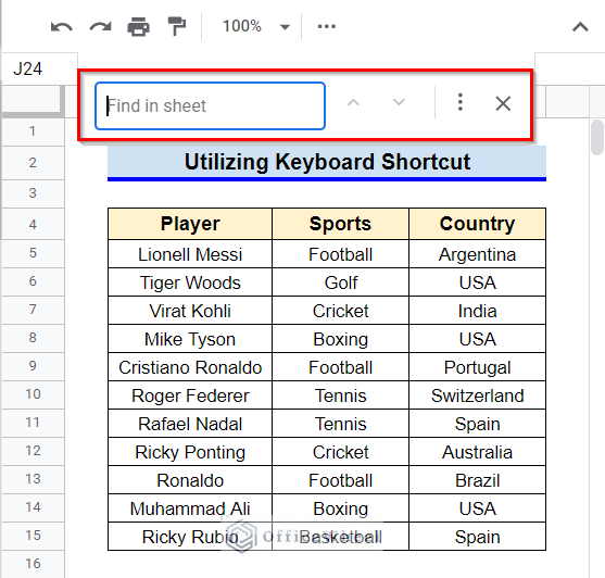
An alternative to using functions for searching information is to use the keyboard shortcut CTRL+F. Although, this search will not be as dynamic as the one with functions. It’s a built-in command, so it won’t create any search box in the sheet.
Steps:
- Open your datasheet and type CTRL+F to open a search box like the following.
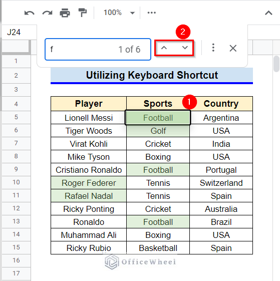
- Type the search key in the search box. As soon as you type the first letter, all the cells that contain that letter, are highlighted in green. The first occurrence is also highlighted with a black order box. You can use the up arrow and down arrow options to move from one result to the next.
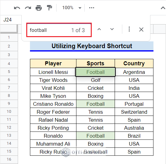
- Finally, if you enter the total search key, only the cells that contain that search key is highlighted.
Read More: How to Search in All Sheets in Google Sheets (An Easy Guide)
Things to Be Considered
- During Data Validation, carefully input the options for the search box. If grammatical mistakes occur, the QUERY function won’t execute properly.
- Remember to put a comma (,) between the list options in Data Validation.
- The functions QUERY and MATCH are case-sensitive, whereas the functions FILTER and FIND are not.
Conclusion
This concludes our article to learn how to create a search box in Google Sheets. I hope the mentioned methods were helpful for your requirements. Feel free to share your thoughts on the article in the comment box.