
Today we will look at how to sum multiple rows in Google Sheets. While one method is expectedly common, the others may prove to help in some dynamic datasets. ...

Today, we will look at how to add up a column in Google Sheets. It is the most common form of calculation that any user does in a spreadsheet. But that does ...

At a professional level, spreadsheet searches can get quite complex with the amount of varying data they might have. Thus, we have to look for viable and quick ...

Today, we will look at how to perform a match from multiple columns in Google Sheets. This process is useful if you want to extract values based on multiple ...

We are already aware of how powerful the INDEX-MATCH combination is when extracting data in Google Sheets. If not, please visit our Using INDEX MATCH in Google ...

Find and Replace can be quite a powerful tool when used in large documents. Its uses are many and, in this article, we will look at how to use Find and Replace ...
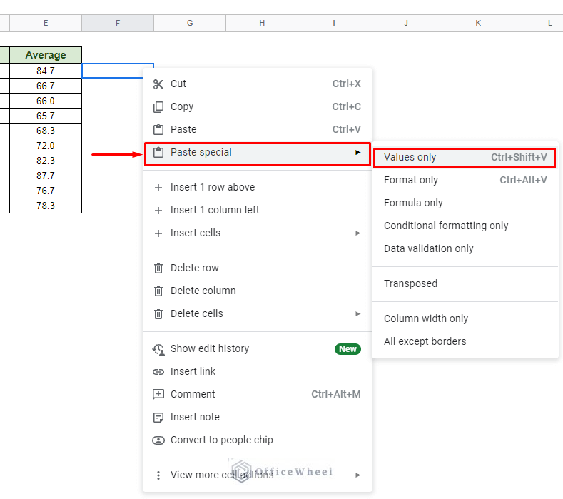
While formulas are the backbone of any professional spreadsheet, I can sometimes be wise to replace formula with raw value in Google Sheets if nothing else but ...
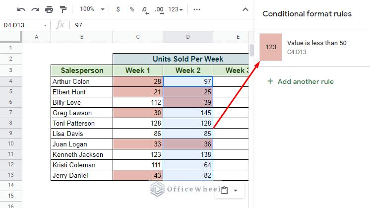
Today we will have a look at how to use conditional formatting in Google Sheets, which is potentially one of the most used built-in functions by any level of ...
Knowing how to copy formatting comes in handy especially when you have multiple worksheets or spreadsheets that have a similar data layout. It will save a ...
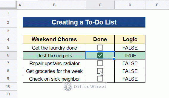
Today, we will look at how we can use Conditional Formatting with a Checkbox in Google Sheets. Conditional Formatting and Checkboxes are widely used in this ...
When we think about multiple conditions, the first thing that comes to mind is its logical formatting. So it comes to no surprise that when creating custom ...
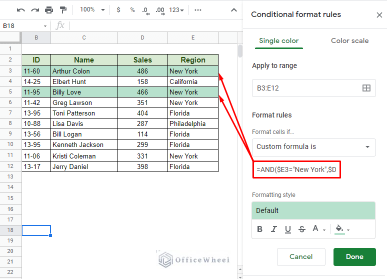
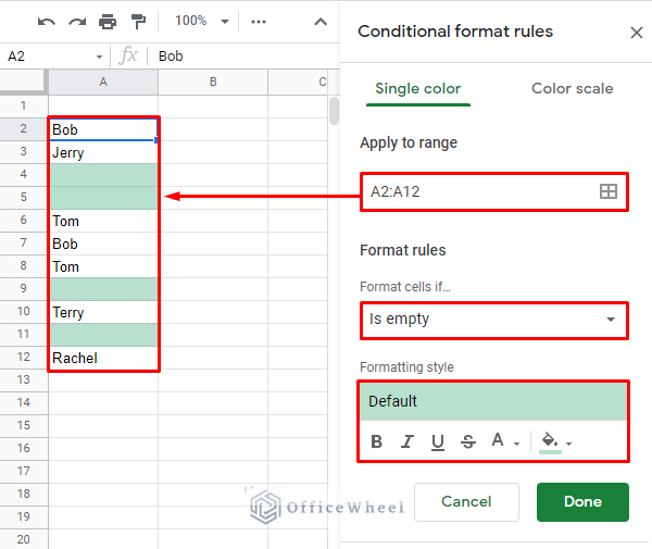
Conditional formatting is quite a versatile function in any spreadsheet application. And today we will see the conditional formatting of a row/rows based on a ...
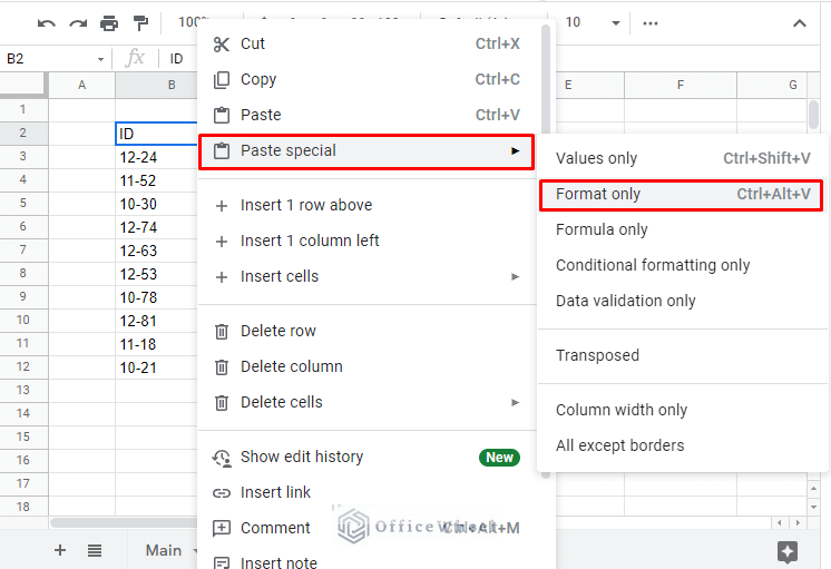
Today, we will look at two very easy ways to copy conditional formatting in Google Sheets step-by-step. We will also see how we can apply these methods when ...
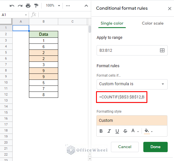
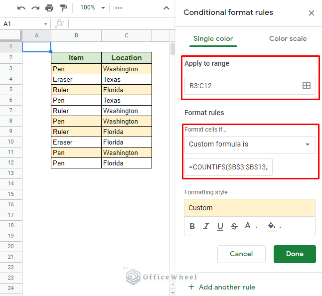
Today we will look at how we can use conditional formatting with custom formula in Google Sheets. Let’s get started. Basics of Using Custom Formula in ...

It is not uncommon that a spreadsheet user may need to apply custom conditions for sorting and organizing data. Understanding that, we will look at how we can ...
- « Previous Page
- 1
- …
- 8
- 9
- 10
- 11
- 12
- …
- 14
- Next Page »
Hello,
If you want to specify which column’s changes will trigger the timestamp, all you have to do is include an IF ELSE statement inside the existing one. For example, let’s say that the SL column is Column A in the sheet:
if(sheetName == 'Stock'){
    if(range.getColumn() !== 1) return
    else{
      var new_date = new Date();
   spreadSheet.getActiveSheet().getRange(row,4).setValue(new_date).setNumberFormat("MM/dd/yyyy hh:mm:ss");
    }
}
So, if changes are made to any column other than column A or 1, no timestamps will be triggered.
For multiple triggers, we recommend different scripts for each.
I hope it helps!
Hi Max,
I am assuming that you are thinking about extracting the letters ABC from ABC-123. In this case, you can approach it in two ways without even using wildcards.
The first way is to use text functions to extract the number of characters from the string:
=LEFT(B2,LEN(B2)-4)
The LEN(B2)-4 removes the last 4 characters from the string.
For a more dynamic approach, you can look for the hyphen/dash as a delimiter to remove characters before or after it. In this case, to get ABC from ABC-123, the formula will be:
=MID(B2,1,FIND(“-“,B2)-1)
Just replace “-” with any delimiter of your choosing.
However, if you still want to extract using regular expression to get ABC from ABC-123, use this:
=REGEXREPLACE(B2,”[0-9-]”,””)
The regular expression to remove all digits and hyphens is given by [0-9-].
I hope this helps!