Data validation will assist you in decreasing the chances of error in your Google Sheets spreadsheet by only accepting acceptable data. For cells in Google Sheets, data validation accepts a specific type or range of data, creates a drop-down list, and alerts you if you enter any incorrect data. In this article, we will show you 2 quick ways of making data validation from another sheet in Google Sheets.
2 Quick Ways to Use Data Validation in Google Sheets from Another Sheet
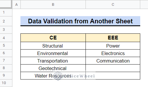
The dataset below will be used to demonstrate the example of making data validation from another sheet in Google Sheets. The dataset contains all the major subjects offered by CE and EEE departments of a university.
1. Create Drop-Down List from Another Sheet
Data validation is a process that can create drop-down lists. Drop-down lists are incredibly helpful since they guarantee that only true information is entered into the cells. Drop-down lists also make it incredibly simple and quick to choose the appropriate text and insert data into cells. First, we will create two independent drop-down lists here for the department and major subject by taking data from another sheet.
Steps:
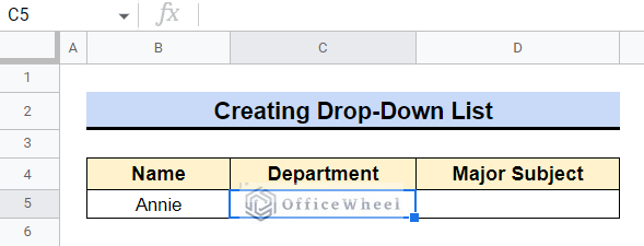
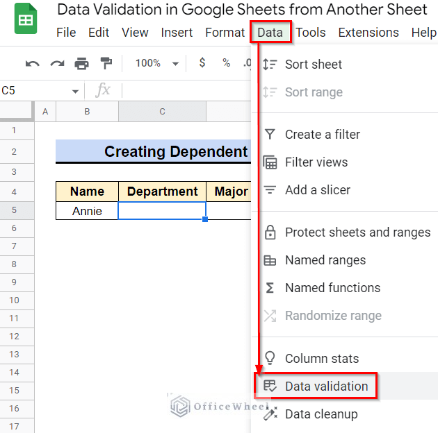
- First, select the cell where you want to create the drop-down list. We chose Cell C5.
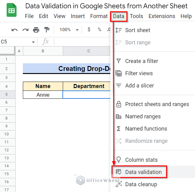
- Now, go to the Data tab from the top toolbar and select Data validation.
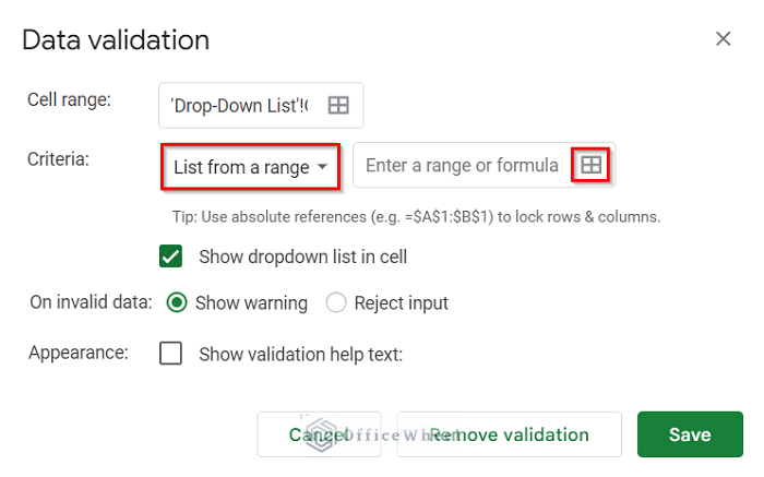
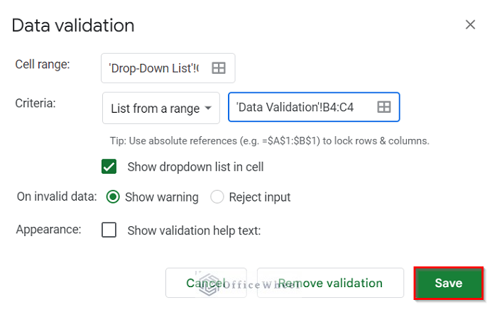
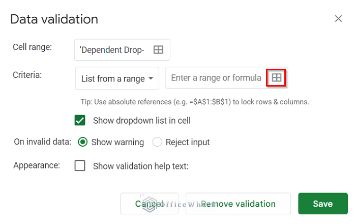
- A Data validation dialog box will open up. Under the Criteria region, choose List from a range and then enter the range by clicking the box icon.
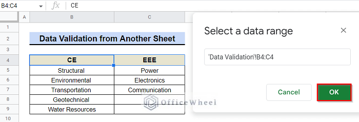
- Select the data range that you wish to see below the drop-down list. In our case, we have selected Cell B4:C4, which is located on another sheet. You should simply type the sheet’s name inside quotation marks, then enter an exclamation mark (!), and then type your data range; or you can just select the data range from another sheet. After selecting the data range, click OK.
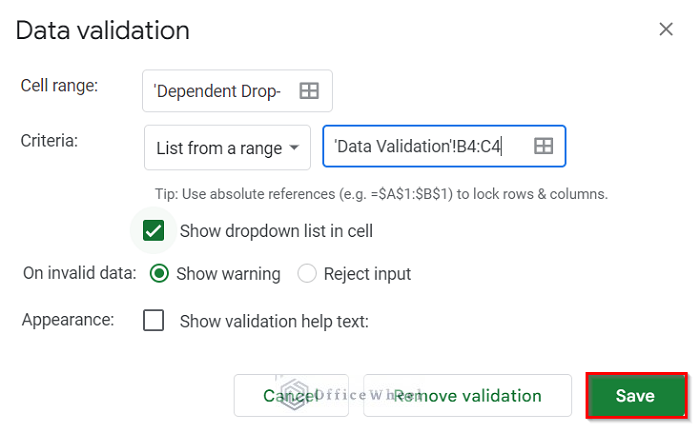
- Now, you can choose either Show warning or Reject input for invalid data. Click Save.
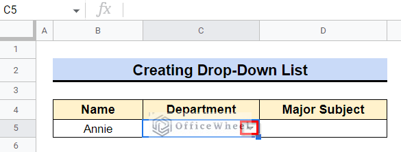
- The drop-down list is created on your desired cell. Click on the drop-down icon.
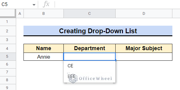
- You can see the data range that you selected to show.
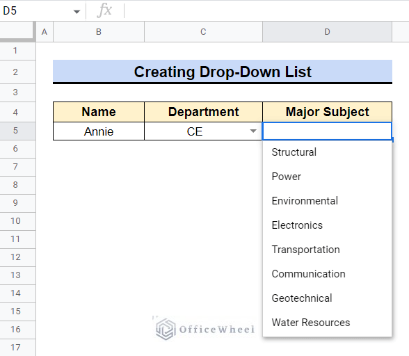
- Similarly, we can make a drop-down list for major subjects also, where we selected all the major subjects as data range.
Look, the second drop-down list is independent because it’s showing all the major subjects, not according to the selection of the first drop-down list. The next method will show you how to make a dependent drop-down list.
Read More: Create Drop Down List in Google Sheets from Another Sheet
Similar Readings
- How to Add Color to Drop Down List in Google Sheets (Easy Steps)
- Use VLOOKUP with Drop Down List in Google Sheets
- How To Lock Rows In Google Sheets (2 Easy Ways)
2. Generate Dependent Drop-Down List from Another Sheet
Creating a dependent drop-down list is essential as after making a choice in one drop-down list, the next drop-down only displays choices that are pertinent to the prior choice. In our dataset, we want to select the department first, then we want to select the major subject based on the department choice.
Steps:
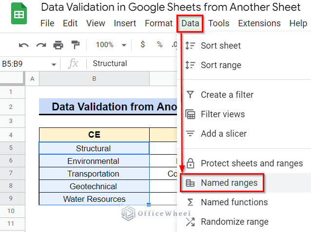
- First, select the major subjects of each department and make a named range for them. We selected Cell B5:B9. Now go to the Data bar from the top toolbar and select Named ranges.
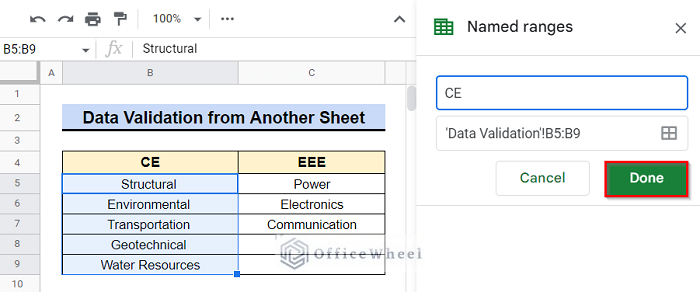
- A Named ranges dialog box will open up. Give it a name. We named it CE. Now click on Done.
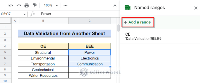
- Again, select the major subjects of the EEE department and click on Add a range.
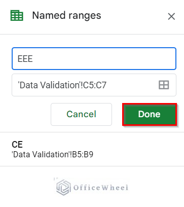
- Again, the Named ranges dialog box will open up. We named it EEE. Then click Done.
- Select the cell where you want the first drop-down list to show. It is for the departments. We selected Cell C5. Now go to the Data tab from the top toolbar and select Data validation.
- Enter the data range that you want to show below the drop-down list.
- We selected Cell B4:C4 which is located on another sheet and click OK.
- Click on the Save option.
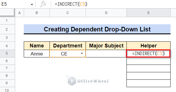
- One drop-down list will be created. To create another drop-down list that is dependent on the first one, we will need a helper column where we’ll apply the INDIRECT function. Select Cell E5 from the helper column and type the formula below-
=INDIRECT(C5)Where C5 is the cell where the first drop-down list is created.
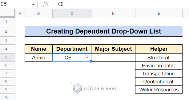
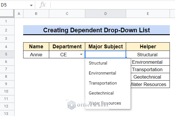
- If we select CE from the first drop-down list, the helper column will show all the major subjects offered by the CE department.
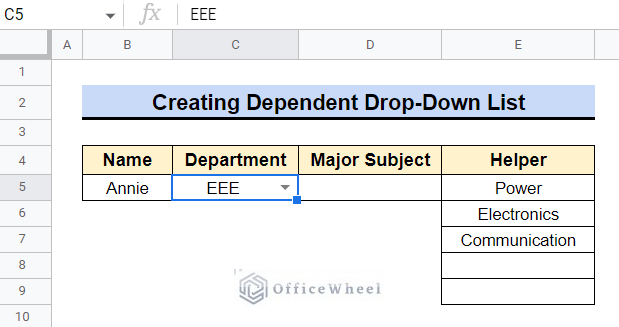
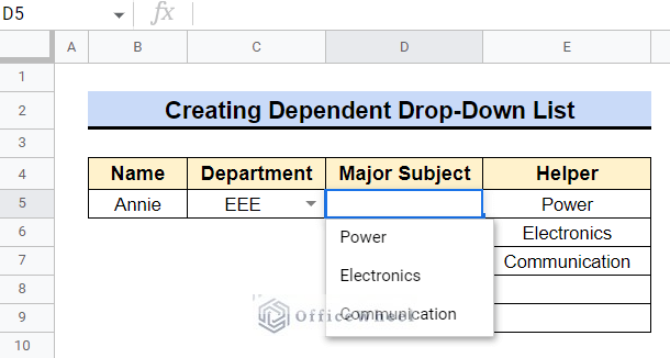
- If we select EEE from the first drop-down list, the helper column will show all the major subjects offered by the EEE department.
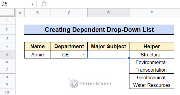
- Now, select a cell where you want your second drop-down list to show. We selected Cell D5.
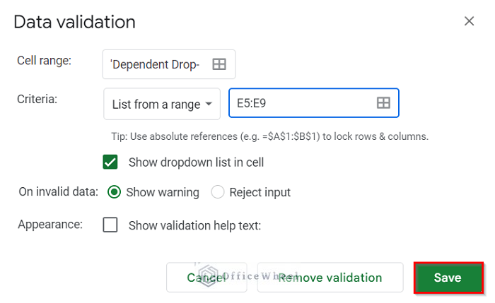
- Following the previously mentioned steps, select the data range for Data validation. We selected the helper column as data range. Then click OK.
- Now, click Save.
- We are done, now you will get your desired list. If you select CE from the first drop-down list, the second drop-down list will show you all the major subjects offered by the CE department.
- And if you select EEE from the first drop-down list, the second drop-down list will show you all the major subjects offered by the EEE department.
Read More: Create Multiple Dependent Drop Down List in Google Sheets
How to Edit Drop-Down List of Data Validation in Google Sheets
After making a drop-down list, you may wish to edit the drop-down list, such as you may want to change the data range. It can also be done in Google Sheets.
Steps:
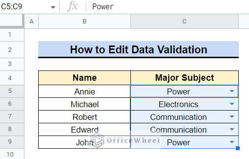
- Select all the drop-down lists containing cells that you want to edit. We selected Cell C5:C9.
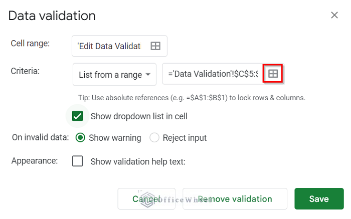
- Go to the Data validation dialog box following the aforementioned steps, and click on the box icon of data range.
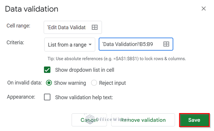
- Select the new data range and click OK.
- Now, click on the Save option.
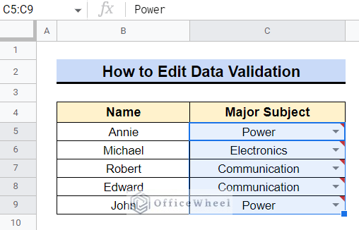
- All the drop-down lists are marked in red as they contain wrong data.
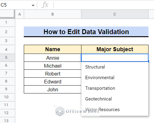
- If you click on the drop-down list, it will show you the new data range.
Read More: How to Edit Data Validation in Google Sheets (With Easy Steps)
How to Remove Data Validation from Google Sheets
At times, you may want to get rid of the Data validation. However, the drop-down list in that cell still exists even after you choose the cell that contains the drop-down list and press the Delete button. Here, we’ll show you how to remove Data validation in Google Sheets.
Steps:
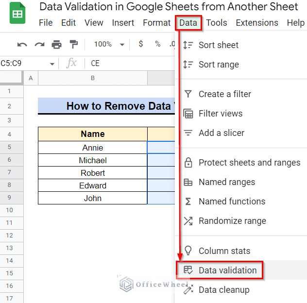
- Choose every cell from which you want to eliminate Data validation. We selected Cell C5. Now go to the Data tab from the top toolbar and select Data validation.
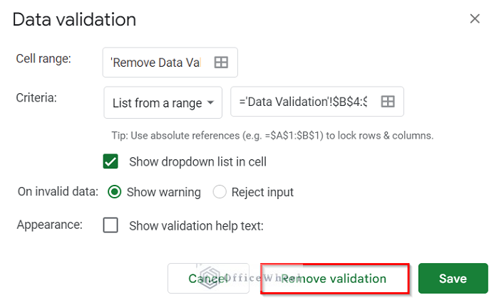
- Click on the Remove validation option.
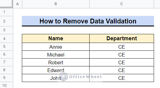
- Now, all the drop-down lists are removed.
Read More: How to Remove Data Validation in Google Sheets
Conclusion
Data validation makes it easier for you to select the appropriate text and swiftly enter data into cells. In this article, we have shown you how to create a simple drop-down list and how to create a dependent drop-down list from another sheet. We have also shown you how to edit and remove data validation from the sheet. We hope this will help you to make data validation from another sheet. Please feel free to leave any questions or suggestions in the comments section below. Visit our site, Officewheel.com to explore more.
Related Articles
- How to Insert a Drop-Down List in Google Sheets (2 Easy Ways)
- Multi Row Dynamic Dependent Drop Down List in Google Sheets
- How to Edit Drop-Down List in Google Sheets
- Create Drop Down List for Multiple Selection in Google Sheets
- How to Create Conditional Drop Down List in Google Sheets
- Updating Cell Values Based on Selection in Drop Down List in Google Spreadsheet

