Applying Filter with REGEXMATCH Function in Google Sheets (Easy Examples)

The REGEXMATCH function of Google Sheets can help us easily filter for text conditions. Not only that but also thanks to the use of regular expressions, multiple text conditions can also be applied.

Let’s see how it’s done.

Table of Contents

The REGEXMATCH Function and its Uses in Google Sheets

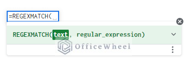
The REGEXMATCH function primarily checks whether a piece of text in a cell matches the given regular expression.

The function’s syntax:

REGEXMATCH(text, regular_expression)

This gives the user great freedom to look for certain text combinations over a large dataset.

The REGEXMATCH function obviously takes advantage of the customizability of regular expressions.

The following table shows all the regular expression symbols (known as metacharacters) that can be used alongside the text conditions:

Characters	What it Does
^	The start of the string
$	The end of the string
.	A single character
+	Character repeats one or more times
\|	The OR logical operator
()	This holds metacharacters. Follows the sequence of characters inside it
[]	Holds characters regardless of sequence

The REGEXMATCH function can be used for multiple spreadsheet processes like categorizing keywords and URLs and simple keyword searches among others. But in this article, we will use REGEXMATCH to search and filter entries from a dataset by matching specific text conditions.

Applying a Filter with the REGEXMATCH Function in Google Sheets

1. REGEXMATCH with the FILTER Function

The simplest way to use REGEXMATCH for a filter is using it alongside, you guessed it, the FILTER function.

The FILTER function takes filter conditions along with the data range, which the REGEXMATCH function can cover.

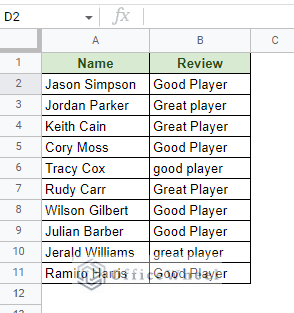
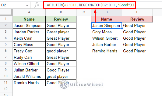
For example, here we have a sample dataset from which we want to filter the entries that contain the Review “Good”:

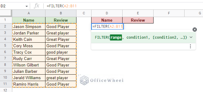
Step 1: Open the FILTER function and apply the data range. Note that all conditions of the FILTER function must come from within this range.

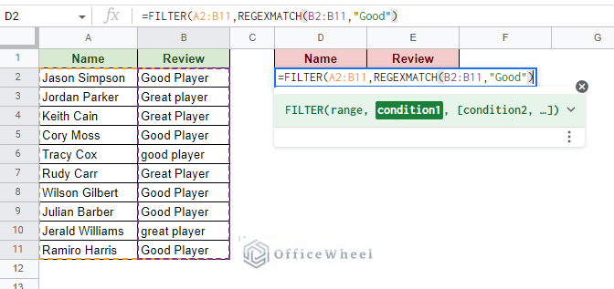
Step 2: For the condition field, we will use the REGEXMATCH formula to search and match for “Good”.

REGEXMATCH(B2:B11,"Good")

Step 3: Close parentheses and press ENTER to apply the filter.

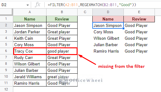
=FILTER(A2:B11,REGEXMATCH(B2:B11,"Good"))

It is important to note that REGEXMATCH is case-sensitive. You will notice in the image above that the Reviews with “good” were not presented in the filter.

Here’s how we can make the filter case-insensitive:

Making REGEXMATCH + FILTER Case Insensitive

We need to do just two things:

Transform the data range values to the lower/upper case.
Search for the lower/upper case of the value in the formula.

For this example, we will search for the lower-case value.

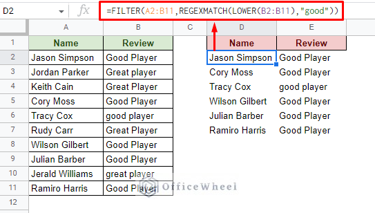
To set the data range to lowercase, use the LOWER function. And then, search for “good” as the regular expression criteria.

The formula:

=FILTER(A2:B11,REGEXMATCH(LOWER(B2:B11),"good"))

Note: We can also use the UPPER function to search with an upper-case value. In that case, set the search word to “GOOD”.

Filter with Multiple Criteria with the OR or AND Logic in FILTER Function

An advantage of using the FILTER function to filter data in Google Sheets is that it can take multiple criteria in the same formula. And that too in both the AND and OR logical conditions.

Thanks to us being able to apply regular expressions through the REGEXMATCH function, we can apply an OR logic filter by using only a single condition field of the FILTER function.

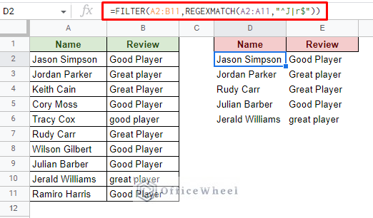
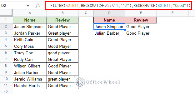
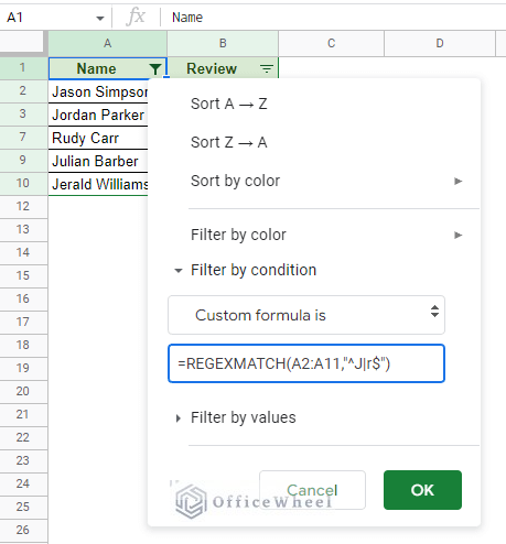
For example, let’s say we want to filter all entries with Names that start with a “J” or end with an “r”.

Recalling the regular expression for string start (^) and string end ($), the formula will be:

=FILTER(A2:B11,REGEXMATCH(A2:A11,”^J|r$”))

As for filtering for multiple AND logic criteria, we can utilize the different condition fields of the FILTER function.

=FILTER(A2:B11,REGEXMATCH(A2:A11,"^J"),REGEXMATCH(B2:B11,"Good"))

As you can see, the AND version of the filter is not limited to a single column for criteria.

Similar Readings

2. REGEXMATCH Function with the Default Filter Feature of Google Sheets

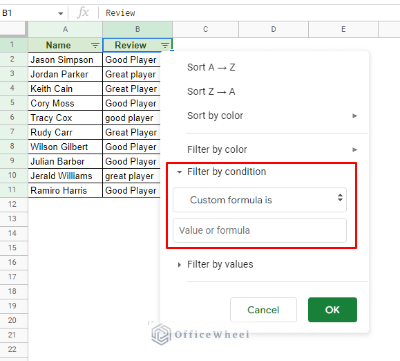
You can also apply the REGEXMATCH function in the default filter of Google Sheets as a custom formula.

While the default filter of Google Sheets has a few compelling ways to apply conditions, the custom formulas will always trump them in terms of customizability.

Like the FILTER function, REGEXMATCH conditions can be directly applied to the custom formula field after applying the default filter on the dataset.

Filter > Filter by condition > Custom formula is

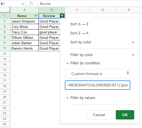
1. For filtering out only “good” players:

=REGEXMATCH(LOWER(B2:B11),"good")

2. The name starts with “J” or ends with “r”:

=REGEXMATCH(A2:A11,"^J|r$")

You get the idea.

Final Words

That concludes all the ways we can use the REGEXMATCH function to filter in Google Sheets. We hope the methods we’ve discussed here come in handy for all your filtering needs.

Feel free to leave any queries or advice you might have for us in the comments section below.