For a wide range of data, repetition is a significant problem. To get rid of this, you must find the duplicates for further analysis. This article can be a lifesaver for you, as we will go through a detailed discussion about how to search for duplicates in Google Sheets.
A Sample of Practice Spreadsheet
You can copy the spreadsheet that we’ve used to prepare this article:
3 Quick Ways to Search for Duplicates in Google Sheets
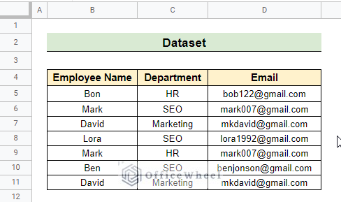
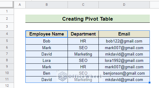
If you follow any of these methods, duplicate searching will be much easier and time optimistic. Before describing any method, let’s know about the dataset that we used. Here, we add three columns that represent the Employee name, Department, and Email.
Now start to explore different methods with good examples.
1. Applying Conditional Formatting
Conditional formatting is a special feature of Google Sheets that allows us to present datasets properly based on rules or criteria. By using this feature, you not only search or highlight the duplicates but also change into the bold, italic format, customize color, and so on. For searching for duplicates in the dataset here, we apply the single-column and multi-column formatting process.
1.1 For Single Column
The most common way to search for duplicates is to apply Conditional Formatting. In this method, you can search for duplicate values from a single column.
Steps:
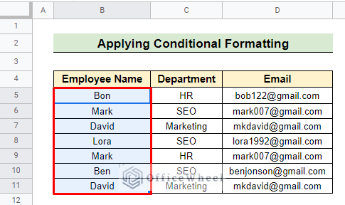
- First, go to your spreadsheet and select a column where you want to search for duplicates.
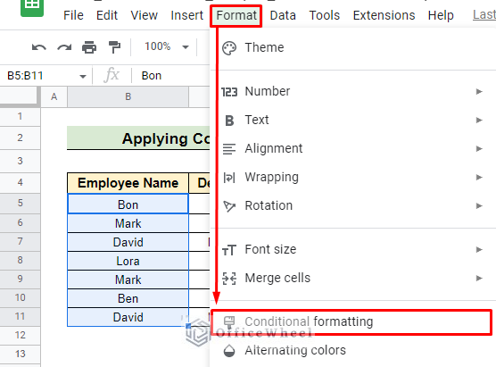
- Then go to the Format bar and select the Conditional formatting option.
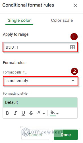
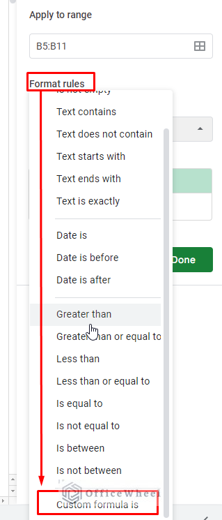
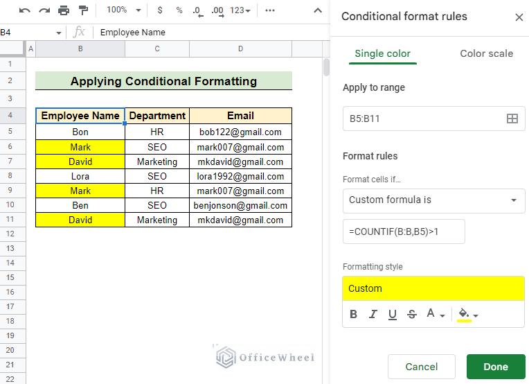
- In conditional format rules, select the data range and press the Format rules option to customize it.
- Select the Custom formula as rule to operate.
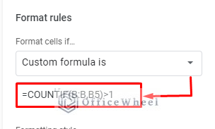
- Insert the formula in the formula bar.
=COUNTIF(B:B,B5)>1Formula Breakdown
- COUNTIF(B:B,B5)>1: The COUNTIF Function will go through the B:B range for all the data present in this column. It starts with B5 cell.
- B:B,B5: Represents all the data in column B.
- (B:B,B5)>1: This checks if the value which appears more than one time in the column.
- COUNTIF(B:B,B5)>1: Marks the duplicates present in the B column.
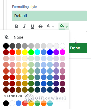
- After that, you can customize the color for indication and choose any colors from the list. It is totally a minor step.
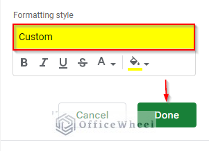
- I chose the yellow color to highlight. Finally, press the Done.
- Go to the main dataset and you will find the duplicate data highlighted with yellow color.
1.2 Multiple Rows & Columns
In this method, you can go through the same procedure as the Single Column method. The change mainly occurs in the formula.
Steps:
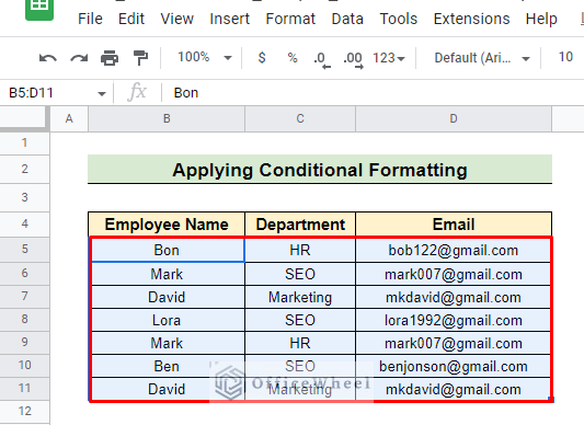
- First, you select the columns from where you want to search the duplicates.
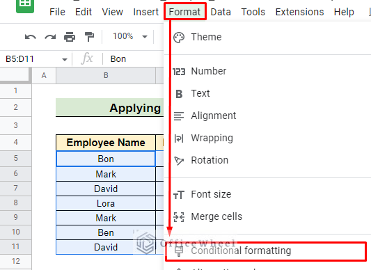
- Go to the Format bar and select Conditional formatting.
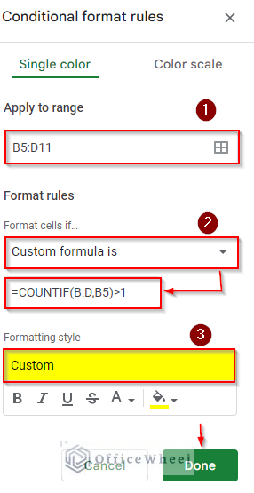
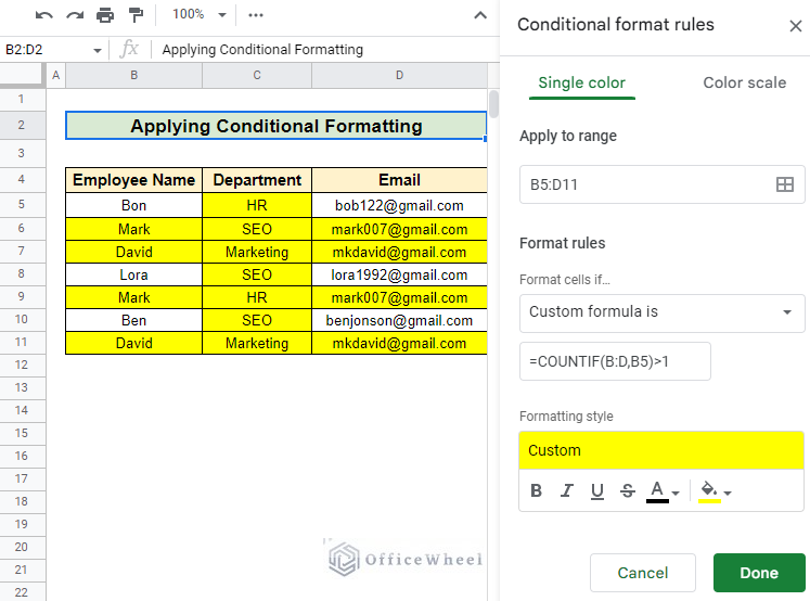
- In conditional formatting, select the range first. The range will be the entire dataset or the column you want to add for searching duplicates. Select the range B5:D11. Then go to the Format rules. Select Custom formula is option. Insert the formula in value or formula bar:
=COUNTIF(B:D,B5)>1Formula Breakdown
- COUNTIF(B:D,B5)>1: The COUNTIF Function will go through the B:D range for all the data present in this table. It starts with B5 cell.
- B:D,B5 represents all the data from columns B to D.
- (B:D,B5)>1 presents the value which appears more than one time in the column.
- COUNTIF(B:D,B5)>1 marks the duplicates present in the entire table.
- Apply or customize the color press Done. After completing the process, you can see the final result in the entire dataset.
Read More: How to Search in a Column in Google Sheets (3 Suitable Ways)
2. Using UNIQUE Function
You can also use the formula technique to search for duplicates in Google Sheets. You can use it in columns or rows and can find the duplicate result in a new column in your sheet. The UNIQUE function helps to find the unrepeated value from the dataset.
Steps:
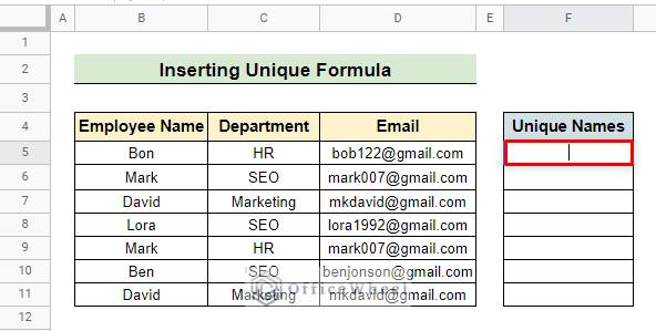
- Open the worksheet and select an empty cell to insert the formula.
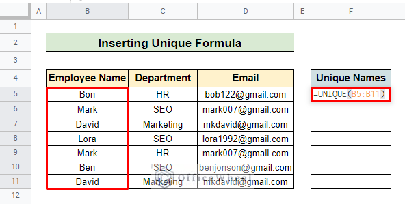
- Then insert the UNIQUE formula and for range select your desired column. Here, we select the Employee Name column to run the method. The selected range is B5:B11.
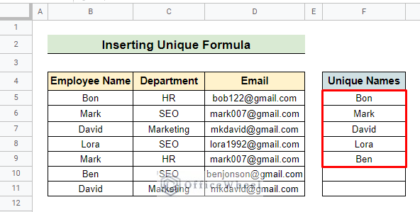
- Press the ENTER key and you will find the unique value in the column. With the help of these, you can easily find out duplicates from Google Sheets.
Read More: How to Use SEARCH Function in Google Sheets (5 Examples)
3. Creating Pivot Table
By using a Pivot Table, you can also search for duplicates in your dataset. Creating a pivot table is more convenient to find out duplicates in the easiest way because it helps you to observe your data very closely. Here are the steps of how to find duplicates through the pivot table.
Steps:
- Select the entire dataset to apply the method.
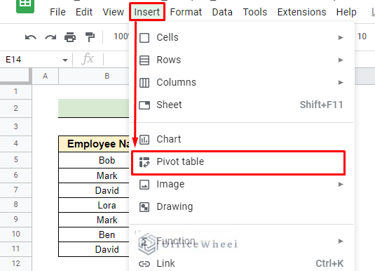
- Go to Insert and select Pivot table.
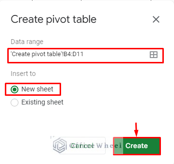
- For creating a Pivot table first, select the data range and then select a new sheet. Then click Create.
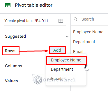
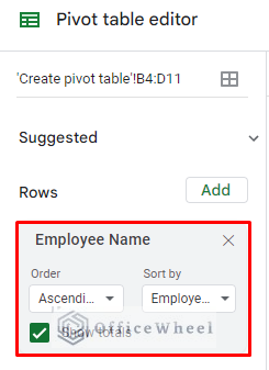
- In the pivot table editor, you can select your row value from any of the selected data.
- We select the Employee Name as our row.
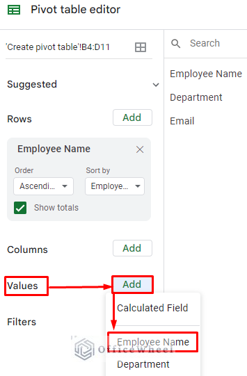
- Then the same column as above for the Value.
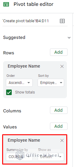
- Selecting the value, set it to summarize by COUNTA or COUNT criteria which should be selected by default.
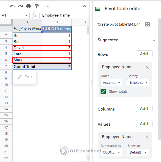
- You can see that the new pivot table finds out all the duplicate values for that column.
Things to Remember
- You have to insert the range carefully when applying the conditional formatting.
- You must input the UNIQUE formula in a new cell.
Conclusion
I hope now you can search for your duplicates in Google Sheets easily, by following any of these methods. If you find any difficulties, feel free to comment and also visit OfficeWheel to explore more.

