Using Conditional Format to Compare Two Columns in Google Sheets

Today we are going to specifically look at how to compare two columns using conditional formatting in Google Sheets.

Let’s get started.

2 Scenarios Where We Compare Two Columns Using Conditional Formatting in Google Sheets

1. Exact Match Rows Between Two Columns using Conditional Formatting in Google Sheets

We start with something simple, that is to highlight the exact row matches between two columns in Google Sheets.

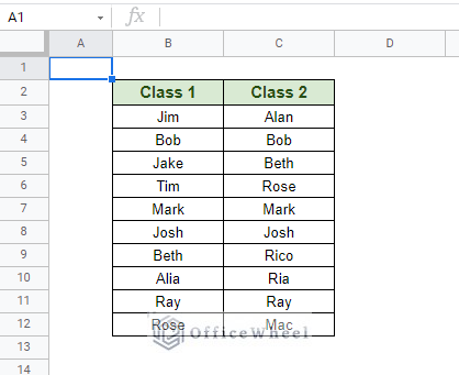
Let’s establish the formula before we apply the conditional formatting for the following dataset.

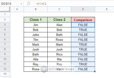
For our test case to be TRUE, both cells in each row must match. This can be done with a simple “equal-to” operation:

Do this for the rest of the rows.

Now that we have established the logic of our comparison, we can move on to apply conditional formatting to highlight the matching rows.

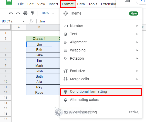
We first select the range of data, cell B3 to C12, and navigate to the Conditional Formatting menu. Format > Conditional formatting

In the conditional formatting rules menu, set up the following conditions:

1. Make sure that the range selected covers all the values that are to be formatted.
2. Select the “Custom formula is” option from the Format rules section.

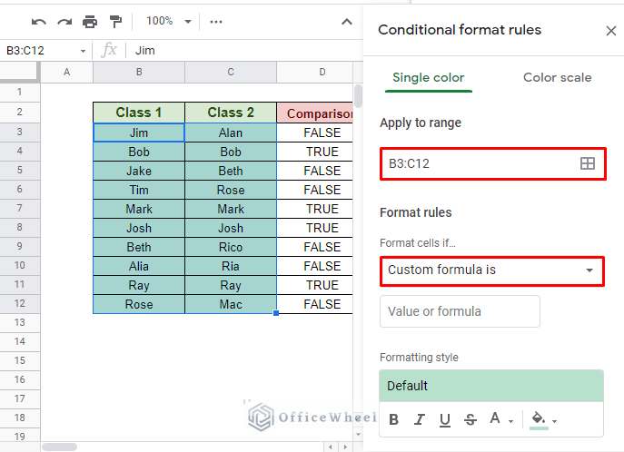
Here we apply the custom formula:

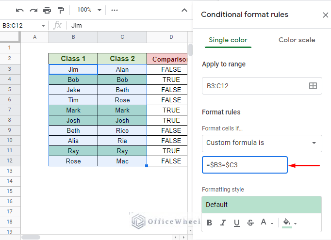
The absolute ($) added in front of column B and C references mean that the columns are fixed whereas the row references are free to move, thus the formatting is painted across the entire row.

As we can see, the matching rows of the two columns have been highlighted. To learn more about this method and much more, please visit our Google Sheets: Conditional Formatting Row Based on Cell article.

2. Compare Between Two Columns to Highlight Occurrences

Comparison between two columns is not limited to exact row matches but much more. One of the other ways that we use column comparison is to find the number of occurrences.

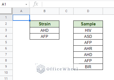
For our example, we will try to find the presence of the Strain from a Sample. This is summarized in the following dataset:

Let’s first develop our formula. We are comparing two columns in Google Sheets where we will match the occurrences of values in one column in the other. For this, we require the COUNTIF function.

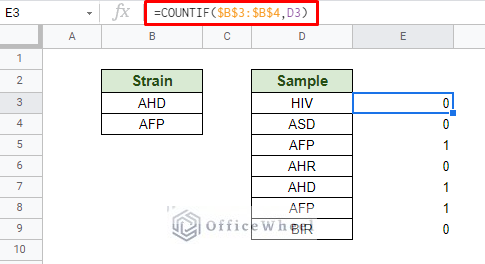
For any matches found, the count value will be 1. But since conditional formatting takes a Boolean value, we must add an IF condition to the formula. This can simply be done by inserting the “>0” condition.

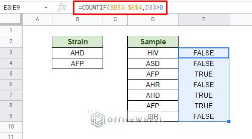
Now, let’s transfer our formula to conditional formatting as a custom formula. Make sure the application range is correct as well.

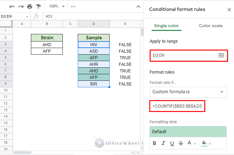
We have correctly compared two columns and highlighted the occurrences of values of one column in Google Sheets.

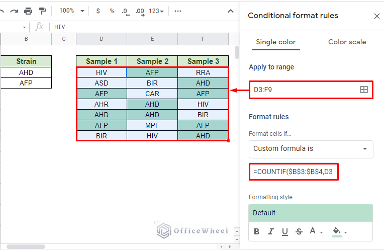
The same formula can be applied to multiple columns to highlight matching data in them as well. The only difference is the range of application:

Read More: Compare Two Columns for Duplicates in Google Sheets (3 Easy Ways)

Final Words

That concludes all the ways we can use conditional formatting to compare two columns in Google Sheets.  However, if you are looking to know beyond the conditional formatting constraints and more about comparing two columns, please see our Compare Two Columns in Google Sheets article.

We hope that our discussion has come in handy. Please feel free to leave any queries or advice you might have in the comments section below.

Related Articles

• How to Compare Text in Google Sheets (3 Easy Ways)