How to Transpose Columns to Rows in Google Sheets (3 Methods)

We are quite familiar with the process of transposing columns to rows in Google Sheets. In this article, I’ll show 3 suitable methods to transpose columns to rows in Google Sheets. I’ll also discuss how to switch columns and how to flip data or rows in Google Sheets. We’ll also see what to do when Paste Transpose isn’t working.

A Sample of Practice Spreadsheet

You can download Google Sheets from here and practice very quickly.

3 Easy Methods to Transpose Columns to Rows in Google Sheets

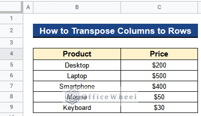
Let’s get introduced to our dataset first. We have some products in Column B and their price in Column C. Now we want to transpose these columns to rows in Google Sheets. I’ll show you 3 simple methods to transpose columns to rows in Google Sheets.

1. Using Paste Special Command to Transpose with Formatting

Initially, we want to transpose columns to rows by keeping their original format. We can do that easily by simply applying the Paste Special Command.

Steps:

• Firstly select the range of data and copy it by pressing Ctrl+C.
• Secondly, select the cell where you want to paste transpose, we chose Cell B11 and give Right-Click on the mouse.
• Then, go to Paste special > Transposed.

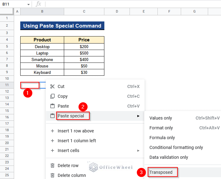
• Lastly, you’ll get the values transposed to rows with formatting.

2. Inserting TRANSPOSE Function

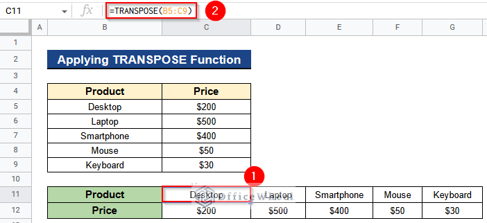
We can also use the TRANSPOSE function to transpose columns to rows in google sheets. The formula is pretty straightforward and gives results immediately. But if we use the formula then we’ll not get the previous format. We have to format our data manually.

Steps:

• First of all type the following formula in Cell C11–

• Then, press Enter to get the values transposed to rows from columns.

Read More: Transpose Multiple Rows into One Column in Google Sheets

3. Assigning Apps Script

Google sheets has a dynamic Extension called Apps Script. We can put some codes in the Apps Script Extension and get the result quickly. The same problem lies here like method 2. We’ll get the result without formatting.

Steps:

• At first, go to Extensions > Apps Script.

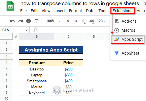
• Next, rename the file as Transposing Values, type the following code, and Click Run.

function transposing() {
var ts = SpreadsheetApp.getActiveSpreadsheet();
var dataset = ts.getActiveSheet()
var values = dataset.getRange(4, 2, dataset.getLastRow(),
dataset.getLastColumn()).getValues();
trans = [];
for(var column = 0; column < values[0].length; column++){
trans[column] = [];
for(var row = 0; row < values.length; row++){
trans[column][row] = values[row][column];
}
}
dataset.getRange(11, 2, trans.length, trans[0].length)
.setValues(trans);
}

• In the end, you’ll get the values transposed to rows without formatting. So we applied the formatting manually after transposing.

How to Switch Columns in Google Sheets

Sometimes we need to switch a column with another column. Here in our dataset, we need to switch Column B that have products with Column C which have Prices. We can do this procedure with a mouse by Drag and Drop method. Let’s see how to do it.

Steps:

• Before all, select Column B and Drag it to the right side with the help of a mouse.

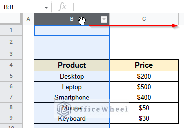
• Finally, you’ll see Column B and Column C switched their place.

How to Flip Data or Row in Google Sheets

Now, we want to flip data or rows in google sheets. It means the transposing too but as we discussed already, so here we’ll discuss a different kind of flipping. For this purpose, we can use the Sort range command. We’ll sort our data alphabetically from A to Z.

Steps:

• Before, Select the data range which is from Cell B5 to Cell C9.
• After, Go to Data > Sort range > Sort range by Column B ( A to Z).

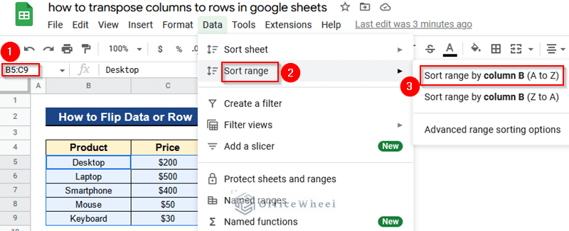
• Ultimately, the values will be sorted alphabetically with respect to Column B.

What to Do When Paste Transpose Is Not Working in Google Sheets?

Once in a while, we’ll find a problem when using the TRANSPOSE function. Like in the following case when we put the formula in Cell C11, it shows #REF! Error. Because we have a value Remark in Cell D11 like the following picture, and that’s why it doesn’t get enough place to paste the transpose values.

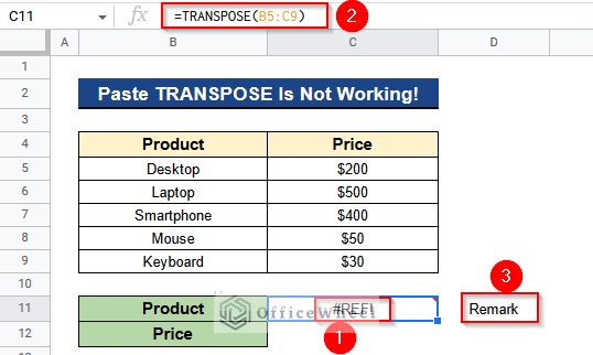
When we put our mouse pointer in Cell C11 it will show an error message.

When we remove the value from Cell D11 the formula will work fine like method 2.

Conclusion

That’s all for now. Thank you for reading this article. In this article, we have learned different procedures to transpose columns to rows in Google Sheets. We have also learned about switching columns and flipping data in Google Sheets. Please comment in the comment section if you have any queries about this article. You will also find different articles related to google sheets on our officewheel.com. Visit the site and explore more.