Every cell in your specified data range is applied with a single formula via the ARRAYFORMULA function in Google Sheets. By converting your formula into an array, the function enables you to create a single formula and apply it to several rows. We can use the ARRAYFORMULA function to sum in Google Sheets. In this article, I will demonstrate 5 simple examples of using the ARRAYFORMULA function to sum in Google Sheets.
5 Simple Examples to Sum Using ARRAYFORMULA in Google Sheets
First, we will use the combination of the ARRAYFORMULA and SUM functions to sum in Google Sheets. Then we will use the ARRAYFORMULA function in two ways to get the sum of multiple columns. Then we will use ARRAYFORMULA to sum based on single criteria and multiple criteria in Google Sheets.
1. Combining ARRAYFORMULA and SUM Functions
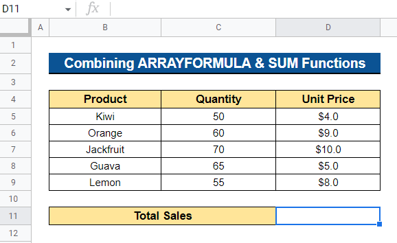
In Google Sheets, we may sum using the ARRAYFORMULA and SUM functions together. Let’s say we have a list of products with quantity and unit prices and want to determine the total amount of sales.
Steps:
- First, select a cell where you want to display the total sales of the products. We selected Cell D11.
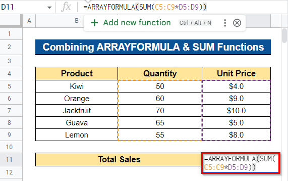
- Now, type the formula below and press the Enter button-
=ARRAYFORMULA(SUM(C5:C9*D5:D9))Formula Breakdown
- SUM(C5:C9*D5:D9)
It will sum up the results of C5:C9*D5:D9.
- ARRAYFORMULA(SUM(C5:C9*D5:D9))
It will return the non-array operations with arrays.
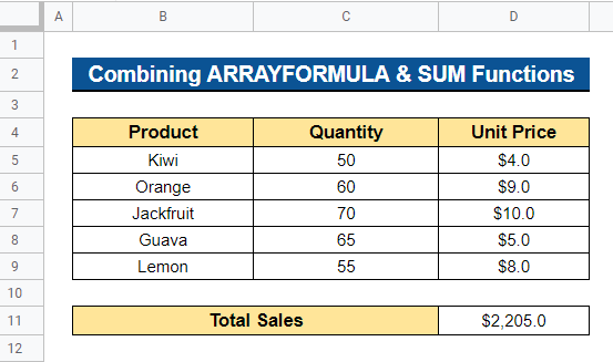
- Thus, it will display the total amount of sales in your desired cell.
Read More: How to Use ARRAYFORMULA with IF Function in Google Sheets
2. Using ARRAYFORMULA to Sum Multiple Columns
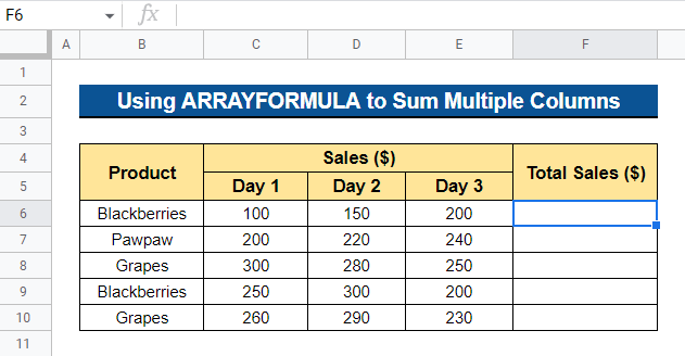
We can sum multiple columns using the ARRAYFORMULA function in Google Sheets. This is a basic formula, to sum up, multiple columns. When there are not many columns to sum, this performs wonderfully.
Steps:
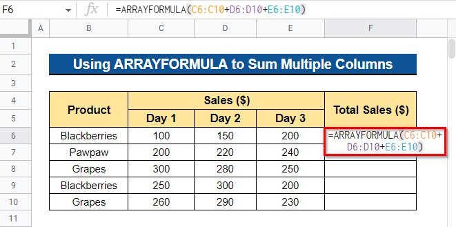
- First, choose a cell where you want to show the sum of total sales. We chose Cell F6.
- Now, enter the following formula and hit the Enter button-
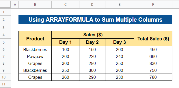
=ARRAYFORMULA(C6:C10+D6:D10+E6:E10)- It will show the total sales of each product right away when you hit the Enter button.
3. Applying MMULT Function to Sum Multiple Columns
We can apply the MMULT function along with the ARRAYFORMULA function to sum multiple columns in Google Sheets. The MMULT function in Google Sheets is likely the most effective approach to calculating the sum of many columns.
Steps:
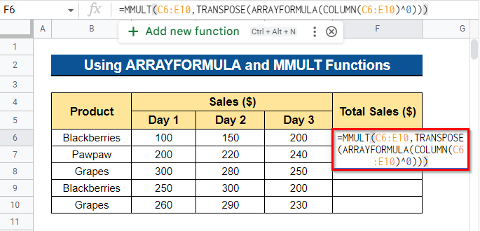
- To begin, select a cell where you want to display the sum of total sales. In our case, we selected Cell F6.
- Now, type the following formula and press Enter–
=MMULT(C6:E10,TRANSPOSE(ARRAYFORMULA(COLUMN(C6:E10)^0)))Formula Breakdown
- COLUMN(C6:E10)
First, it will return the column number of your data range.
- ARRAYFORMULA(COLUMN(C6:E10)^0)
Then, the ARRAYFORMULA function will return the non-array functions into an array.
- TRANSPOSE(ARRAYFORMULA(COLUMN(C6:E10)^0))
After that, the TRANSPOSE function will transpose the rows and columns of the array.
- MMULT(C6:E10,TRANSPOSE(ARRAYFORMULA(COLUMN(C6:E10)^0)))
The MMULT function then determines the matrix product of two supplied matrices in the form of arrays or ranges.
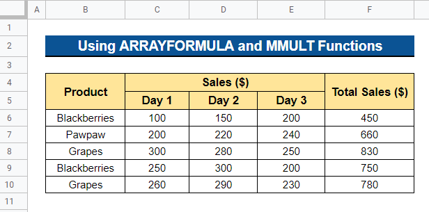
- The total sales of each product will be shown as soon as you hit the Enter button.
Read More: How to Highlight Duplicates for Multiple Columns in Google Sheets
4. Coupling SUMIF and ARRAYFORMULA
In Google Sheets, we may sum by combining the SUMIF and ARRAYFORMULA functions. When summing numbers based on one criterion, SUMIF is utilized.
Steps:
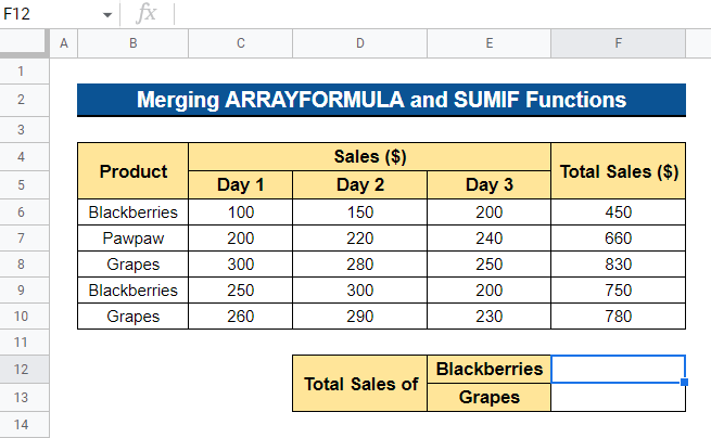
- We want to know the total sales of Blackberries and Grapes. To do this, first select a cell where you want to display the output. We selected Cell F12.
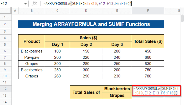
- Now, type the formula below and hit the Enter key-
=ARRAYFORMULA(SUMIF(B6:B10,E12:E13,F6:F10))Formula Breakdown
- SUMIF(B6:B10,E12:E13,F6:F10)
It returns the conditional sum across Cell F6:F10 based on the condition given by Cell E12:E13 across the range Cell F6:F10.
- ARRAYFORMULA(SUMIF(B6:B10,E12:E13,F6:F10))
It will return the non-array operations into an array.
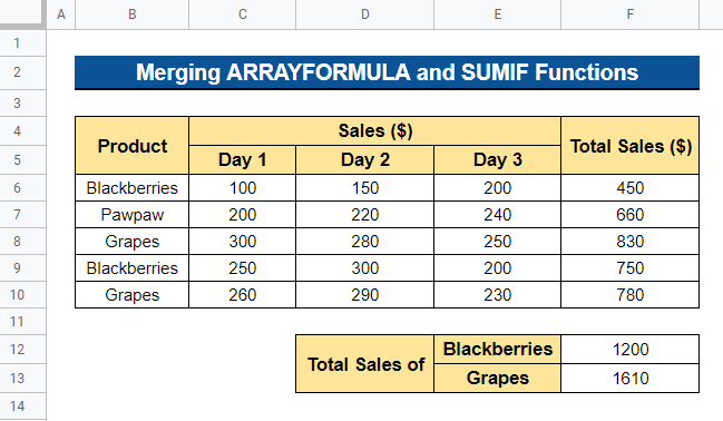
- Thus, it will display the total sales of Blackberries and Grapes.
5. Merging SUMIFS and ARRAYFORMULA
To sum up, in Google Sheets, we may also combine the SUMIFS and ARRAYFORMULA functions. Summarizing data in a range based on several criteria is the goal of the SUMIFS function.
Steps:
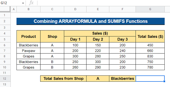
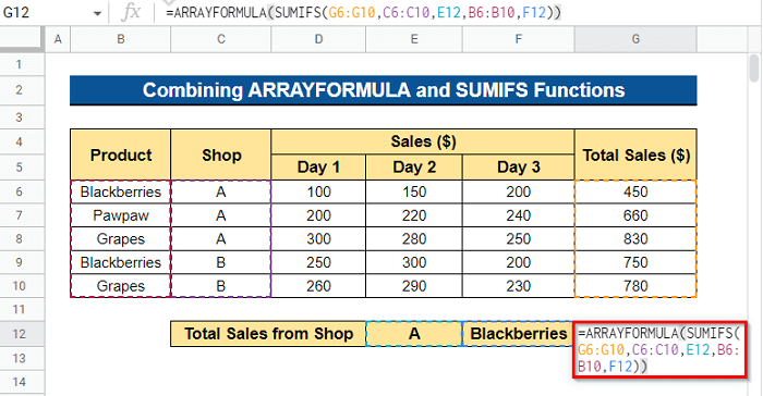
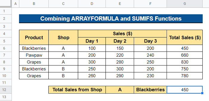
- We’re interested in seeing how many Blackberries are sold overall by Shop A. To display the output in a cell, you must first select it. We chose Cell F12.
- Now, enter the following formula and hit Enter–
=ARRAYFORMULA(SUMIFS(G6:G10,C6:C10,E12,B6:B10,F12))Formula Breakdown
- SUMIFS(G6:G10,C6:C10,E12,B6:B10,F12)
Based on a variety of criteria, it will give the sum of a range.
- ARRAYFORMULA(SUMIFS(G6:G10,C6:C10,E12,B6:B10,F12))
It will give back the non-array operations into an array.
- Thus, it will show the total sales of Blackberries from Shop A.
What to Do If ARRAYFORMULA Is Not Working in Google Sheets?
The ARRAYFORMULA function in Google Sheets may be used to sum and return values for the sum over all rows. However, if you use the ARRAYFORMULA incorrectly, it can display an error, or the value might only be entered into one row rather than all the rows. Here, I’ll give you an example.
Steps:
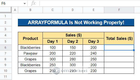
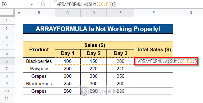
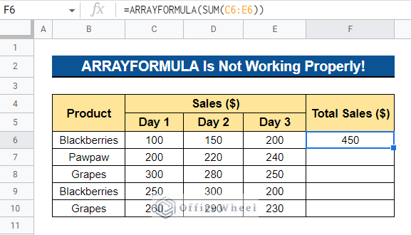
- We want to get the total sales of each product. So, we selected Cell F6.
- Now, if you enter the formula below to sum the multiple columns and press Enter–
=ARRAYFORMULA(SUM(C6:E6))- It will show the total sales for one row only. But we wanted to know the total sales for every product.
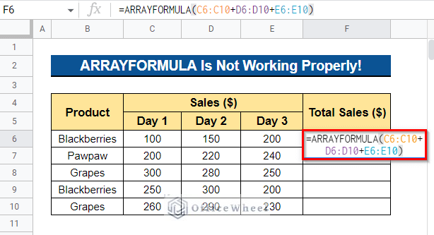
- To achieve this, first clear the cell. Then enter the formula below and press Enter–
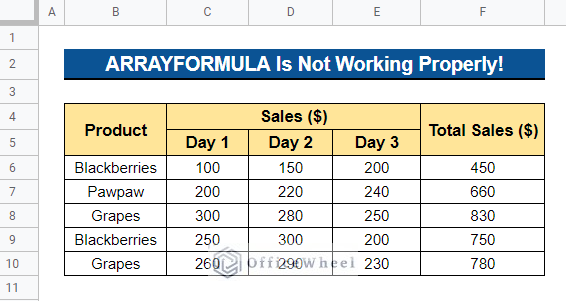
=ARRAYFORMULA(C6:C10+D6:D10+E6:E10)- Thus, it will display the total sales for each product.
Conclusion
In this article, I have shown 5 simple examples, to sum up by using the ARRAYFORMULA function in Google Sheets. I have also shown what to do if the ARRAYFORMULA function is not working properly in Google Sheets. Please feel free to ask any questions or comment on any ideas in the comment section below. To explore more, visit Officewheel.com.
Related Articles
- How to Use ARRAYFORMULA with VLOOKUP in Google Sheets
- COUNTIF Contains Text in Google Sheets (4 Ways)
- How to Merge Columns in Google Sheets
- Use IF and OR Formula in Google Sheets (2 Examples)
- How to Link Cells Between Tabs in Google Sheets (2 Examples)
- Use RIGHT Function in Google Sheets (6 Suitable Examples)

