How to Filter by Condition Using a Custom Formula in Google Sheets (3 Easy Examples)

Using a custom formula is the easiest way to filter by a specific condition in Google Sheets.

While the filter feature has improved by leaps and bounds, sometimes complex user requirements can only be tackled using a custom formula.

In this article, we will look at why and how we apply a custom formula to filter in the spreadsheet application.

Table of Contents

How to Filter by Condition Using a Custom Formula in Google Sheets

Why do we need to use Custom Formulas to Filter?

The basic filter feature of Google Sheets already has a wide choice of conditions.

Even with all these options, a user can still face certain limitations:

The filter feature cannot work with multiple conditions. You can only choose one option among all that is presented in the menu.
The filter feature cannot reference cells as a condition. Cell referencing is a core process of any spreadsheet. Many filter requirements depend on the values of other cells in the worksheet.

The only way to overcome these limitations is by using a custom formula depending on the scenario. This can be done within the default filter feature or as a separate formula in the worksheet.

Let’s see how it’s done with a few examples.

Example 1: Filter by Multiple Number Conditions Using a Custom Formula in Google Sheets

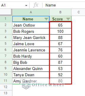
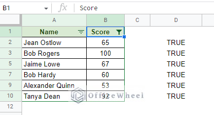
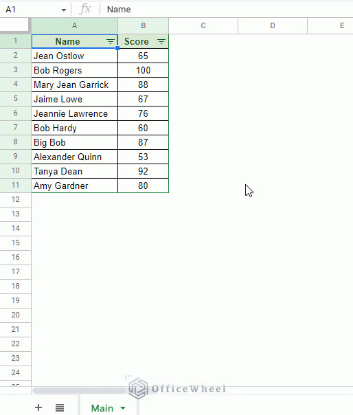
A common filtering requirement is to filter by two or more different number sets in Google Sheets. For example, filter the following dataset for scores under 70 or scores over 90.

In the traditional filter, we could’ve only applied one condition. That is not the case if we create a custom formula.

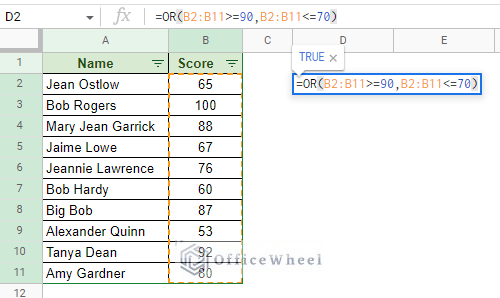
Step 1: We have two conditions, and we want either of them to be TRUE. Thus, we require a formula with the OR logic. Luckily, we have the OR function to do that.

Step 2: The two conditions mentioned are “less than or equal to 70” and “greater than or equal to 90”. Here’s the formula where the OR function incorporates these two conditions.

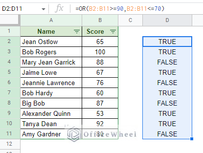
=OR(B2:B11>=90,B2:B11<=70)

The result:

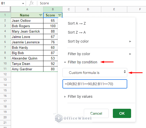
Step 3: Now that we have the formula generated, it’s time to apply it to the filter. Open the filter menu of the Score column and navigate to the “Custom formula is” option.

Filter > Filter by condition > Custom formula is (at the bottom)

Enter the custom formula in the field here.

Step 4: Press OK to apply.

Example 2: Filter by Cell Reference Value using Custom Formula In Google Sheets (Contains Text)

Cell references are crucial when it comes to setting up dynamic conditions. However, this cannot be done using the default filter menu. Thus, custom formulas come to the rescue.

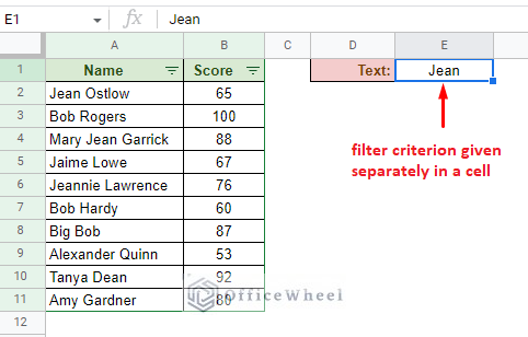
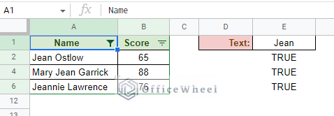
For example, instead of typing in a filter criterion each time, let’s say it is inputted in a separate cell, as seen in the following image:

Step 1: Just like before, we must first create a suitable formula. Note that this time we are filtering for a text value.

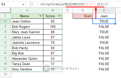
The best way to create a match formula for text is by using regular expressions. In this case, we will use the REGEXMATCH function. The function looks up a range and matches the text in the data range.

REGEXMATCH(A2:A11,$E$1)

Note that the ARRAYFORMULA function is only here to help present all the results of the range at once.

Also, notice that the cell reference for the search criterion is locked with absolutes ($) so that the reference always points to this cell.

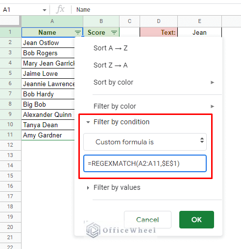
Step 2: Apply the formula (without ARRAYFORMULA) in the “Custom formula is” field.

Step 3: Click OK to apply the filter.

Similar Readings

Example 3: Use the FILTER Function to Overcome Certain Limitations

If you haven’t already noticed, there is an underlying limitation of the previous two methods, methods using the traditional filter feature of Google Sheets. That is the fact that you cannot apply a filter condition beyond a single column.

This further limits the AND logical conditions for filters.

For that, we have a remedy in the form of the FILTER function.

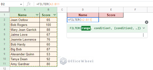
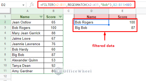
Let’s consider the scenario where we want to filter all entries that contain the name “Bob” and have scored over 80 points.

Step 1: Open the FILTER function and input the data range. Note that the data range will also imply the number of columns that will be extracted during the filter.

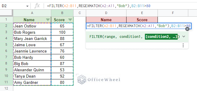
Step 2: Apply the two conditions. The text match condition will once again use the REGEXMATCH function:

REGEXMATCH(A2:A11,"Bob")

The numerical condition does not require any extra functions:

B2:B11>80

Step 3: Close parentheses and press ENTER to apply the filter.

Not only can it take multiple column conditions at once, but the FILTER function also comes with all the other advantages. On top of that, the source dataset is unaffected.

Final Words

That concludes all the ways we can filter by condition using a custom formula in Google Sheets.

The default filter feature of the application has advanced enough to cover most filter criteria. However, user requirements can give rise to complex conditions that can only be achieved by creating a custom formula. This includes the use of the FILTER function.

Feel free to leave any queries or advice you might have in the comments section below.